High-Integrated IP Camera SoC Processor

ISP API Tuning SOP ; Version 1.17

1. OVERVIEW¶

1.1. Module Description¶

The ISP module aims to analyze and process input data from video source. By setting up associated video parameters and conducting camera tuning with this module, users are expected to implement various functions, including black level calibration, lens calibration, 3A and 2D/3D noise reduction, CCM, and Gamma.

1.2. Flow Chart¶

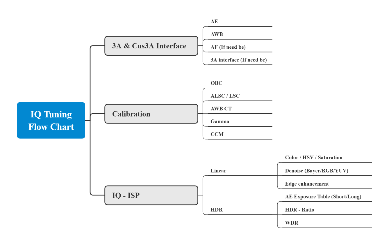
Figure 1-1: IQ Tuning – Flow Chart

2. CALIBRATION¶

Each sensor or lens has its own characteristics. Before use, the sensor or lens should go through calibration and parameter setting process, so that the subsequent image quality adjustment can be properly performed. In the following sections, an introduction of the calibration flow is provided in detail to help you get started with the calibration. We advise that you follow our suggestions when doing the calibration.

2.1. AWB Color Temperature Curve Range Adjustment¶

Although, according to the ISP pipeline, AWB comes after Shading, we recommend doing AWB color temperature curve range adjustment first, and check back later if the AWB color temperature curve range needs to be fine-tuned in response to ALSC calibration result, once available. The reason behind our suggestion is that, shading calibration will require the CCT value estimated by AWB based on statistical data, and besides, the calibration or not of shading has relatively smaller impact on AWB.

2.1.1. Calibration Environment¶

The calibration is to be done using a Macbeth standard light booth, with a gray card occupying the entire screen placed within. If gray card is not available, you can utilize the gray wall inside the light booth to perform the analysis instead.

Before the adjustment, make sure OB has been calibrated and applied correctly.

Moreover, when using the RGB sensor, see to it that the IR cut is well caped.

2.1.2. Calibration Interface¶

Choose Awb AnalyzerCombo from the Select Plugin menu on top of the API tool to open the calibration tool interface.

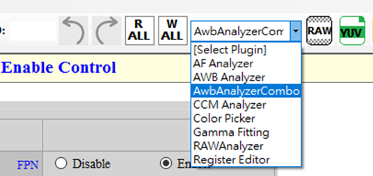
Figure 2-1: Plugin Menu

Figure 2-2: Awb Analyzer Combo Interface

2.1.3. Interface Description¶

Main Window:

Each green dot in the window represents an entry of statistical data.
Ten color temperature ranges are available for adjustment. Please refer to the CT Area table on the right-hand side for the color temperature of each color temperature range. Only those color temperatures which fall within the range encircled in blue in the diagram above are deemed effective color temperatures. Color temperatures outside of that scope will not be taken into account as effective statistics. To adjust the color temperature ranges, click on the control point of the color temperature with your mouse and drag it directly.
The RGain, BGain and the color temperature [CT] that are being calculated will be shown on the upper right corner of the interface.
- File: There are four options:
  1. Load Statistics
  2. Load CTArea
  3. Save Statistics
  4. Save CTArea
- RawFormat: The format for opening raw data. Be sure to set the format before you load statistics from the raw image.
- StartIdx: Start index of effective color temperature range; suggested value is 2.
- EndIdx: End index of effective color temperature range; suggested value is 7.
- Update Live Statis: Updates the statistical data in real-time.
- Reset CTArea: Restores the color temperature range parameter setting to the one currently applied to the platform.
- Apply to Camera: Applies the color temperature range to the platform.

2.1.4. Calibration Steps and Calibration Data Application¶

Set StartIdx and EndIdx to define the color temperature range intended for AWB calibration. We suggest setting StartIdx=2 and EndIdx=7; that is, do AWB calibration when environmental color temperature is somewhere between the range 2300K ~ 10000K.
Prepare a light meter to measure the actual color temperature of the light source to be adjusted.
Press the Update Live Statis button to update the statistics of the current light source, then press “File” → “Save Statistics” to save the statistics. Adjust the color temperature range of the color temperature which is closest to the actual color temperature. The color temperature range can be of a size sufficient to cover most of the statistics. Moreover, be sure the color temperature (CT) estimated via the CT button on the upper right corner is close to and not too dissimilar from the actual color temperature.

Figure 2-3: 2800K Light Source Adjustment Example
Switch to a light source with a different color temperature, and repeat steps 2 and 3. Since the amount of light sources in the light booth is limited and may not cover all of the color temperature curve range, if the color temperature ranges to be adjusted do not have any statistics available for reference, you are suggested to smooth the color temperature curve range based on already adjusted color temperature ranges.
Once the adjustment is done, press “File” → “Save CTArea” to save the adjusted color temperature range, click “Apply to Camera” to apply the setting to the platform, and then close the Awb Analyzer Combo. Go back to the API tool interface and choose “AWBCTCali” on the left-hand side, press the “ReadPage” button to load the setting on the platform back to the camera, and then go to “File” → “Save” → “Bin file” to save the AWB color temperature curve setting to the bin file of the API.

2.1.5. Precautions¶

Proper environment setup of the light booth is a basic requirement for AWB calibration. We hence recommend that you save all light source statistics in the course of adjustment, so that, when fine-tuning of the color temperature curve range is required in a later case, the fine-tuned statistics can be read back to the light booth statistics database to confirm, without going through the trouble of setting up the light booth environment again, whether the white balance of the light booth environment will be adversely affected, thereby saving considerable time. If any AWB scene is in question, you can provide the statistics associated with the scene together with the color temperature range setting used at that time, to allow the responsible engineer to do the analysis.

2.2. AE Exposure Table Setup¶

Different sensors and lens have different characteristics and capabilities. The default AE exposure table is not necessarily suitable for the module used. Here, we suggest that you check the AE exposure table setting and modify the setting, where necessary, to fit the current module.

2.2.1. Adjustment Interface¶

Select AE from the menu on the left-hand side, then click “ExpoTblEntry” to edit the AE exposure table.

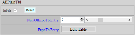
Figure 2-4: AE Setting Interface

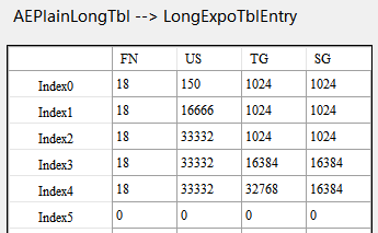
Figure 2-5: AE Exposure Table

2.2.2. Parameter Description¶

NumOfExpoTblEntry : Sets the number of AE exposure tables. Let’s take Figur 2-4 as an example, as the number of AE exposure tables is set to 5, you should fill out 5 sets of AE exposure table correspondingly.

First Column (FN) : Lens aperture value (Fn) x 10. For example, if aperture is 1.6, the value will be 16.

Second Column (US) : Shutter (usec)

Third Column (TG) : Total gain (1024 = x1 gain), i.e. sensor gain x ISP gain

Fourth Column (SG) : Sensor gain (1024 = x1 gain)

2.2.3. Setting Items¶

Verify the lens aperture value, and fill out the value (lens aperture value x10) in the first column.
Verify the maximum gain, then fill the value in the third column of the penultimate row.
If ISP gain is not used, copy the value in the third column to the fourth column.

3. GAMMA FITTING & COLOR CORRECTION¶

Different gamma and color have different impact on noise. Besides, denoise adjustment will be a lot easier if you apply gamma and color settings beforehand. Therefore, gamma and color corrections are normally done first even when they are placed after denoise in the PUDDING pipeline.

3.1. Gamma Fitting¶

Color fitting result is susceptible to differences in brightness. Differences in brightness mainly come from AE and gamma. As such, it is imperative that gamma fitting should be done before color fitting. This step aims to adjust the gamma of the calibration model close to that of the contrast model. Before calibration, make sure the dynamic range is set to full range.

3.1.1. Calibration Environment¶

Prepare an OECF chart and have light illuminated on the chart uniformly. Place the chart in middle of the screen when shooting; do not occupy the whole screen with the chart, otherwise the result might be affected by shading.

Figure 3-1: Shooting Screen Example

3.1.2. Calibration Interface¶

From the Select Plugin menu on top of the API tool, select “Gamma Fitting” to open the calibration tool interface.

Figure 3-2: Gamma Fitting Interface

3.1.3. Calibration Steps¶

Set up the environment, and shoot images required for fitting between calibration model and contrast model. Since exposure may affect brightness, the gamma fitting should be performed based on the same exposure setting. The easiest way to obtain the closest exposure is to set the lightest patch of the OECF chart as close to (but not equal to) 255 as possible when capturing images (RAW for calibration model and JPG for contrast model). The logic is that even though we do not know what the gamma of the contrast model looks like, the lightest patch usually remains unchanged, which makes it a suitable candidate as the base for fitting.

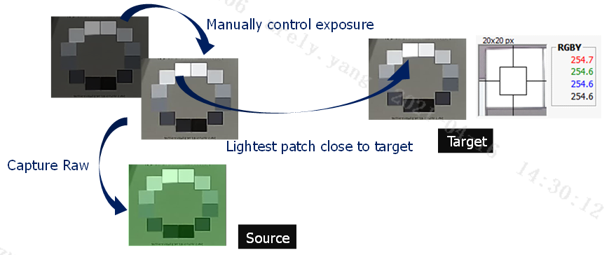
Figure 3-3: Shooting Source and Target Images
Read the OECF patch value of source raw data:
Select Options from the interface tool menu, fill in the correct raw information and OB (WB not required), and click OK.

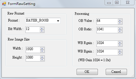
Figure 3-4: Raw Setting Interface

Drag-select OECF patch with your mouse. Be sure each patch is correctly located within the patch location.

Figure 3-5: Drag-Selecting OECF Patch
Read the OECF patch value of target image:

Same as the preceding step; only in this step the target reads image file without setting the raw information.
Set the fitting related parameters. We suggest setting “Patch values” as the value method, and “Exponential” as the fitting method.

Figure 3-6: Gamma Fitting Setting Suggestions
After setup, click “Match GMA” to start gamma fitting. If nothing abnormal is found with the curve generated by the fitting, click “Save GMA” to save the gamma curve. Finally, check to see whether the start and end of the saved gamma curve fall at 0 and 1023, respectively. If not, modify them manually.

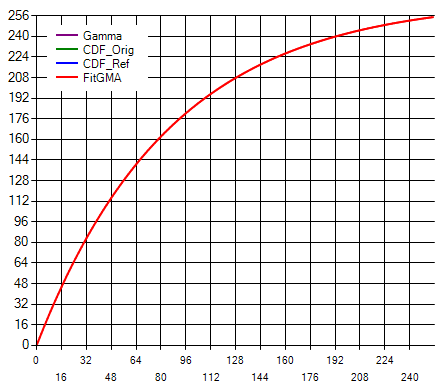
Figure 3-7: Ideal Gamma Curve(Smooth and Incremental)

3.2. Color Correction¶

The main purpose of this step is to bring the color of the calibration model close to that of the contrast model. Color correction involves two parts: the first (and also the most important) part is color matrix fitting; the second part is HSV fine-tuning, which allows you to adjust local color saturation and hue according to your preference. Color matrix and HSV each support up to 16 sets of color temperatures. Index0 through Index15 represent color temperatures from low to high. Be sure to follow this rule when filling in the parameters.

3.2.1. CCM Adjustment¶

After finishing calibration of light sources of various color temperature with the tool, be sure to fill in the results manually in the corresponding CCM fields.

3.2.1.1. Adjustment Interface

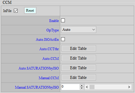
Figure 3-8: CCM Adjustment Interface

3.2.1.2. Parameter Description

ISOActEn : Enables/Disables the function to set CCM as unit matrix automatically at Night mode. If enabled, CCM will automatically be switched to unit matrix when IQMode is Night.

CCTthr : Color temperature node setting. Need to fill in the color temperature value obtained at the time of calibration. CCM and HSV will look to this CCTthr to determine which node setting to apply. When filling out indexes from small to large, the color temperature should follow the low-high sequence. 16 sets of nodes at most are supported. For nodes not used, set them to 0.

CCM : Color matrix setting of each color temperature. Need to fill in the color matrix according to the corresponding color temperature. When filling out indexes from small to large, the color temperature should follow the low-high sequence.
Sum of each row is shown too. If the sum displayed is not 1024, modify the CCM manually.

SATURATIONbyISO : Color matrix saturation adjustment. The procedure will do an interpolation based on this setting between user-defined matrix and unit matrix. Range is 0 ~ 100. 0 means using unit matrix, and 100 means using user-defined CCM. This parameter changes with the gain value.

3.2.2. HSV Adjustment¶

If further color fine-tuning is required after application of the CCM setting, you can use HSV to achieve this. HSV will divide the entire color domain into 24 even parts to allow you to adjust the hue and saturation of each part according to your preference. HSV has same parameters as CCM; that is, they all vary with color temperature, rather than with gain value.

3.2.2.1. Adjustment Interface

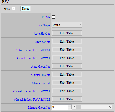
Figure 3-9: HSV Adjustment Interface

3.2.3. Parameter Description¶

HueLut : Allows you to make partial hue adjustment. Parameter range: -64 ~ 64, 0 means no change.

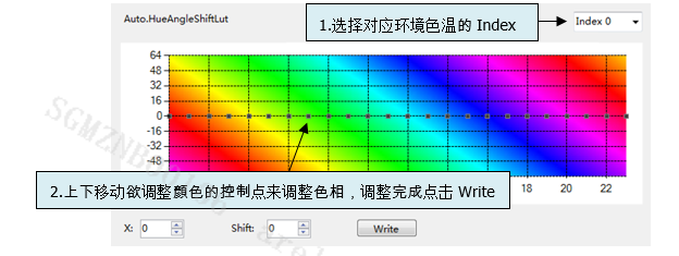
Figure 3-10: Hue Adjustment Interface

SatLut : Allows you to make partial saturation adjustment. Parameter range: 0 ~255, 64 means no change.

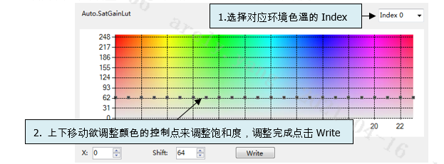
Figure 3-11: Sat Adjustment Interface

HueLut_ForUnitCCM : Allows you to make hue adjustment based on unit matrix. Parameter range: -64 ~ 64, 0 means no change. Parameter switching is based on color temperature.

SatLut_ForUnitCCM : Allows you to make saturation adjustment based on unit matrix. Parameter range: 0 ~ 255, 64 means no change. Parameter switching is based on color temperature.

GlobalSat : Allows you to make global saturation adjustment. Parameter range: 0 ~ 255, 64 means no change. Parameter switching is based on gain value. If the saturation is to be decreased, we suggest using this parameter since it is more effective for noise level reduction; and if the saturation is to be increased, we suggest using the saturation API since it will be less likely to lead to noise level rise.

3.3. Saturation Adjustment¶

UV adjustment based on brightness (Y) and saturation (UV) includes Adjust UV by Y and Adjust UV by UV. It is mainly used to reserve color adjustment flexibility in YUV domain. Besides, since brightness and saturation are independent of each other, you can maintain a fixed brightness while making partial saturation adjustment. When high exposure values are applied to sensor, you can lower the color noise in dark area, or increase/decrease the saturation according to user preference, to make the picture look brighter or softer.

3.3.1. Adjustment Interface¶

Select “Saturation” from the menu on the left-hand side, and then you will find the Saturation interface to the right of your screen.

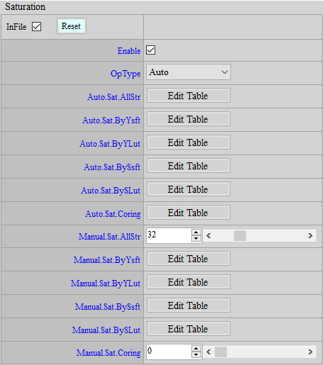
Figure 3-12: Saturation Adjustment Interface

3.3.2. Parameter Description¶

Sat.AllStr : Variable strength of global saturation. Parameter range: 0 ~ 127 (32=1x).

Sat.ByYsft and Sat.BySsft : Can be used to adjust the UV X-axis spacing based on Y/UV with a special limitation to be observed, as stated below:

The nodes are a power of 2 and add up, for example, Sat.ByYSFTAdv[5] = { 3, 3, 5, 7, 7}.

Suppose the first node is 0, the second node will be 0+2^3, the third 0+2^3+2^3, the fourth 0+2^3+2^3+2^5, and so forth.

Then the X-axis spacing is { 0, 8, 16, 48, 176, 255}, where the last node is greater than 255.

The limitation is that, the sum of the first four X-axis nodes must be less than 255, while the last node greater than or equal to 256.

For example, if Sat.ByYsft[5] = {8, 0, 0, 0, 0}, with the first node being 0 and the second 0+2^8=256. This would go against the limitation above.

Sat.ByYLut and Sat.BySLut : The values of the nodes can be decided by the user. As a special application, in the case where HDR function is enabled, causing high brightness to be oversaturated, you can utilize Sat.ByYLut/Sat. BySLut to adjust the high brightness/high saturation UV downward, so that the picture appears more natural under HDR effect.

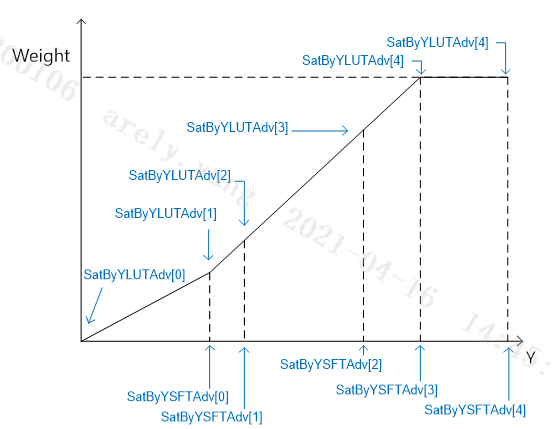
Figure 3-13 Sat.ByYsft[5] & Sat.ByYLut[6]

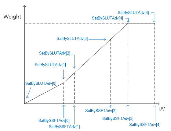
Figure 3-14 Sat.BySsft[5] & Sat.BySLut[6]

4. DENOISE, EDGE ENHANCEMENT & SATURATION¶

Although the default parameters in iqfile will be read into the API tool when the platform is connected to the interface, whether an IP is enabled or disabled will not be shown. As such, if you want to adjust the image quality of a new sensor from scratch, we suggest that you go to the Enable Control interface first to bypass all functions except sharpness and those already adjusted (OB, ALSC, Gamma, and Color) to have a general overview of the sensor’s status before denoise process, such as the maximum resolution supported and whether crosstalk or false color exists. After that, you can enable the function as desired for further adjustment to avoid unnecessary function affecting the overall image quality. Theoretically, sharpness should be bypassed too; however, for the convenience of observation, we recommend that you keep sharpness on and use the following default values (set Over/UnderShootGain to a smaller value if the gain is large, so that the picture does not look too strange).

Figure 4-1: Suggested Sharpness Default Values

When doing adjustment at a high gain without denoise but with sharpness, the picture will appear so noisy that it would be difficult to decipher the effect of adjustment. To solve this issue, we suggest that you set Y.TF.STR to a stronger value to stabilize the picture for the convenience of making other adjustments before adjusting NR3D. The adjustment should preferably be done by following the sequence of ISO index. To prevent parameter interpolation from affecting your judgement, we suggest setting AE to Manual SV mode, with specific gain value assigned to each node, and doing so one after another. Before adjusting image quality, be sure you clean the lens and keep it focused, while ensuring that the IR cut of the RGB sensor is caped.

4.1. Crosstalk & False Color Adjustment¶

Before moving forward to denoise adjustment, check if there is any fixed pattern, cross talk or false color. If any of such phenomena exists, correct it first. For one thing, these functions go before denoise in the pipeline; for another, special phenomenon can only be resolved effectively with specific function. Any attempt to remove these phenomena using denoise might impair the image quality.

4.1.1. Crosstalk (Green Equal)¶

Crosstalk is primarily an issue caused by the compatibility of lens and sensor. When the angle of the light entering the micro lens on the sensor is too large, the signal supposed to be received by certain pixel might be mistakenly received by its neighboring pixel, causing the Gr-Gb imbalance to become greater. This issue tends to occur at the corner of a picture or when the light enters at a certain angle.

4.1.1.1. Phenomenon

A maze/labyrinth pattern appears on screen.

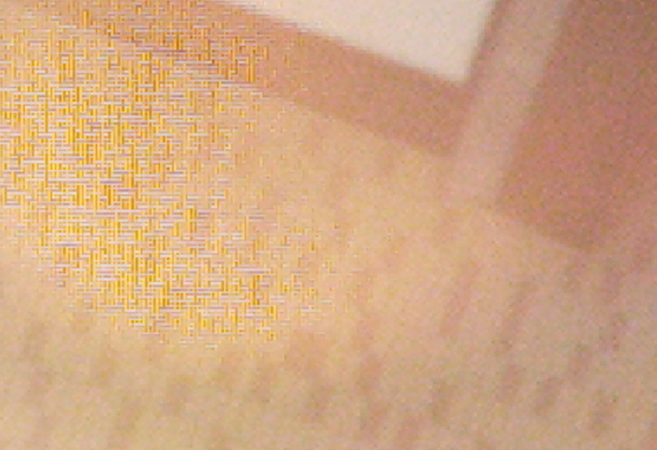
Figure 4-2: Crosstalk-induced Maze/Labyrinth Phenomenon

4.1.1.2. Adjustment Interface

Select “BayerCompensation” from the menu on the left-hand side. You will find the Crosstalk interface to the right of your screen.

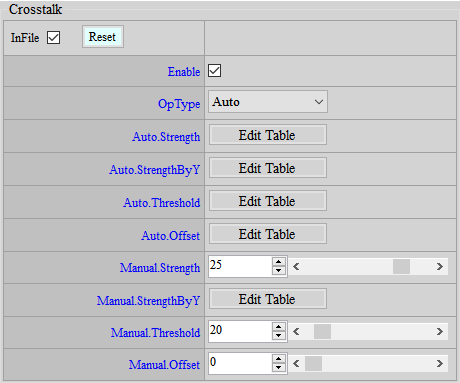
Figure 4-3: Crosstalk Adjustment Interface

4.1.1.3. Parameter Description

Strength : Crosstalk strength value. Parameter range: 0 ~ 31. The greater the strength, the better the effect.

StrengthByY : Adjusts crosstalk strength value by Y. The closer to the right side of the horizontal axis, the brighter. Parameter range: 0 ~ 127. The greater the strength, the better the effect. 64 means no change.

Threshold : Crosstalk threshold ratio value. Parameter range: 0 ~ 255. The larger the value, the wider the range of action.

Offset : Crosstalk threshold offset value. Parameter range: 0 ~ 4095. The larger the value, the wider the range of action.

4.1.1.4. Adjustment Steps

Set Offset to 0 and Threshold to 128, increase Strength from 0 and observe the region where crosstalk needs to be removed and the region where the details should be maintained. Stop when both crosstalk and details are acceptable.
Use Threshold if further fine-tuning is required.
If crosstalk is still obvious in dark region, increase Offset.

4.1.2. False Color¶

False color occurs in cases where direction is not considered, or where direction is considered but misjudged, during demosaic process. This phenomenon normally occurs at the high-frequency region or the edge of a picture.

4.1.2.1. Phenomenon

False color at the high-frequency region or the edge of a picture.

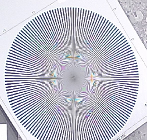
Figure 4-4: False Color Phenomenon

4.1.2.2. Adjustment Interface

Select “BayerCompensation” from the menu on the left-hand side. You will find the AntiFalseColor interface to the right of your screen.

Figure 4-5: False Color Adjustment Interface

4.1.2.3. Parameter Description

FreqThrd : Frequency threshold. Parameter range: 0 ~ 255. The smaller the value, the easier it is to remove false color.

EdgeScoreThrd : Edge threshold. Parameter range: 0 ~ 255. The larger the value, the easier it is to remove false color.

ChromaThrdOfStrengthMax : Maximum strength threshold. Parameter range: 0 ~ 127. The larger the value, the easier it is to reduce saturation in moire region.

ChromaThrdOfStrengthMid : Medium strength threshold. Parameter range: 0 ~ 127. The larger the value, the easier it is to reduce saturation in moire region.

ChromaThrdOfStrengthMin : Minimum strength threshold. Parameter range: 0 ~ 127. The larger the value, the easier it is to reduce saturation in moire region.

StrengthMid : Medium strength. Parameter range: 0 ~ 7. The smaller the value, the lesser the saturation.

StrengthMin : Minimum strength. Parameter range: 0 ~ 7. The smaller the value, the lesser the saturation.

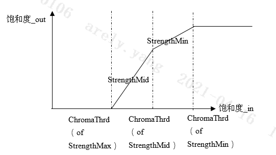
Figure 4-6: False Color Curve

4.1.2.4. Adjustment Steps

IF (freq > FreqThrd && edgeScore < EdgeScoreThrd)

    isMoire = TRUE;

ELSE

    isMoire = FALSE;

The anti-false color function extracts false color at high-frequency region by two conditions: Frequency and Edge Score. During the tuning process, we suggest that you loosen these two conditions, adjust the reduced saturation, and then gradually find out the threshold values of Frequency, Edge and ChromaThrd. If the effect is not satisfactory enough or the side-effect is too apparent, you can modify one or two of the threshold values further.

Set “ChromaThrdOfStrengthMax” and “EdgeScoreThrd” to the maximun, and set “FreqThrd,” “ChromaThrdOfStrengthMid” and “ChromaThrdOfStrengthMin” to the minimum. At this time, the image should be mono color.
Increase the value of “FreqThrd” to restore the color of the whole image back to normal except the false color region. Stop when the false color can be processed and the color of the whole image is basically normal. Write down the FreqThrd value at this point.
Set “FreqThrd” to 0 again. This time, decrease the value of “EdgeScoreThrd” to restore the color of the whole image back to normal except the false color region. Stop when the false color can be processed and the color of the whole image is basically normal. Write down the EdgeScoreThrd value at this point.
Keep “FreqThrd” at 0, and set “EdgeScoreThrd” to the maximun again. Reduce “ChromaThrdOfStrengthMax” to an extent where the color of the whole picture is restored to normal and the false color turns gray. If you cannot have both at the same time, maintaining the color of the whole image is a priority.
Increase “ChromaThrdOfStrengthMid” to make the remaining false color turn lighter. Same as stated above, try at least to keep the color of the whole image normal except the false color region.
Increase “ChromaThrdOfStrengthMin” to further reduce the saturation of remaining false color.
During adjustment, the value of “ChromaThrdOfStrengthMin” should always be larger than that of “ChromaThrdOfStrengthMid,” and “StrengthMid” should be smaller than “StrengthMin.”
Fill in “FreqThrd” and “EdgeScoreThrd” with the previously recorded values.
If there is still side effect in the normal color region, increase FreqThrd or decrease EdgeScoreThrd to restore surroundings to the normal color.
Under the premise that false color can be removed but adjustments of FreqThrd and EdgeScoreThrd would cause side effect, try to decrease FreqThrd as small as possible and increase EdgeScoreThrd as large as possible, and then start reducing ChromaThrdOfStrengthMax or raising the ChromaThrdOfStrengthMid and ChromaThrdOfStrengthMin until the impact of the side effect is acceptable or disappears.

NOTE:

FalseColor will be of some help to thinner purple edges. If purple edges remain serious when FalseColor is set to the strongest strength, you can use HSV to reduce the saturation for the purple hue. During the adjustment, watch out if the saturation of the normal purple object is too low.
Adjustment of false color is highly related to the existence of crosstalk; thus, we suggest that crosstalk tuning to be completed before the anti-false color process.
ChromaThrdOfStrengthMax and ChromaThrdOfStrengthMid represent threshold values of different chroma sources; thus, the tuning of these two parameters is independent of each other. However, ChromaThrdOfStrengthMid and ChromaThrdOfStrengthMin still bear certain corresponding relations; the value of ChromaThrdOfStrengthMid should be lager than that of ChromaThrdOfStrengthMin.

4.1.3. PFC (Purple Fringing Compensation)¶

4.1.3.1. Phenomenon

Purple fringes appear at the edge of an object.

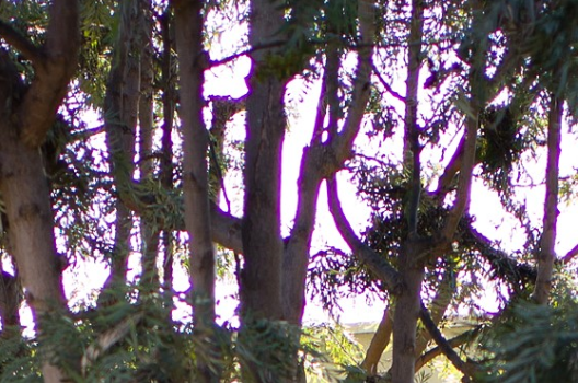
Figure 4-7: Purple Fringing Phenomenon

4.1.3.2. Adjustment Interface

Select PFC from the menu on the left-hand side. You will find the PFC interface to the right of your screen.

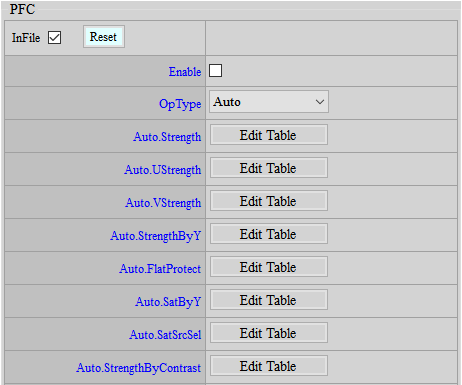
Figure 4-8: PFC Adjustment Interface

Figure 4-9: PFC_EX Adjustment Interface

4.1.3.3. Parameter Description

Strength : Strength of purple fringing compensation. Parameter range: 0 ~ 255. The larger the value, the stronger the de-fringe effect.

UStrength : Strength of de-fringe effect at U channel. Parameter range: 0 ~ 63. The larger the value, the stronger the de-fringe effect.

VStrength : Strength of de-fringe effect at V channel. Parameter range: 0 ~ 63. The larger the value, the stronger the de-fringe effect.

StrengthByY : Purple fringe tends to occur at a darker region surroundeded by a high-brightness region. Hence, we can set different de-fringe strengths against different levels of brightness. Strength at the rightmost side of the horizontal axis represents the brightest. Parameter range: 0 ~ 255. The larger the value, the stronger the de-fringe effect.

FlatProtect : Flat area judgement, to protect large area of purple from being misjudged as purple fringe. Parameter range: 0 ~ 127. The larger the value, the wider the area to be exempt from PFC process.

SatByY : High-contrast area judgement. Since purple fringe normally occurs at a high-contrast area, we can use SatByY[0] to determine the extent of contrast. Parameter range: 0 ~ 25. A larger value means the detected contrast must be greater than SatByY[0] to be recognized as high contrast. SatByY[1] is used to judge the extent of saturation. Parameter range: 0 ~ 25. The larger the value, the brighter the area to be exempt from PFC process.

SarSrcSel : Selects whether or not to do NR treatment in the course of high contrast area judgement. Parament range: 0 ~ 1. 0 means NR treatment not required, and 1 means NR treatment required. We suggest enabling this function in low-contrast cases.

StrengthByContrast : Applies different PFC strengths depending on different levels of contrast. The rightmost end of the horizontal axis represents the highest contrast. Parameter range: 0 ~ 63. The larger the value, the higher the PFC strength.

DbgEn : Scope of PFC. Parameter range: 0 ~ 1. 1 means function enabled.

GSkipEn : Skips PFC treatment against G channel, to avoid fringe loss issue. Parameter range: 0 ~ 1. 1 means function enabled.

SatMaskSel : Selects mask size for contrast area judgement. Parameter range: 0 ~ 1. Mask 0 encompasses a smaller size, and Mask 1 a larger size.

SatAmpEn : When enabled, will increase the precision for contrast area judgement.

StrengthByHue : Applies different PFC strengths depending on dfferent hues.

4.1.3.4. Adjustment Steps

Set SatAmpEn.
Observe the width of purple fringe according to the lens performance, and decide the size of SatMaskSel. If the purple fringe is wider, use a larger mask for compensation first.
Adjust StrengthByY, SatByY, StrengthByContrast, and StrengthByHue based on the brightness area where the purple fringe is located, the extent of contrast, and the color distribution of the purple fringe.
1. StrengthByY: Observe at what brightness the purple fringe occurs. Normally, darker area will be assigned a higher strength setting.
2. SatByY, StrengthByContrast: Observe at what contrast the purple fringe occurs. Normally, higher contrast will be assigned a higher strength setting. SatByY is used to control the fall point of the horizontal axis of the following diagram, and StrengthByContrast is used to control the vertical axis of the following diagram. In low contrast cases, the contrast judgement might have some error due to presence of noise point. So you can relax SatByY[0] a bit to prevent noise point from being misjudged as a high-contrast area.
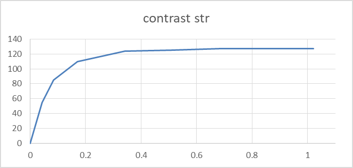
Figure 4-10: Contrast and Strength Parameters
Control FlatProtect, to ensure the flat area will not be subjected to PFC process.
Adjust the final PFC strength. If any particular color is to be treated as a special case, you can apply different UStrength and VStrength settings.

4.1.4. Demosaic¶

4.1.4.1. Phenomenon

Misjudgement of direction and artifacts happen when picture resolution is increased.

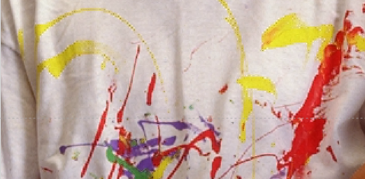
Figure 4-11: Artifacts at the Edge of an Object

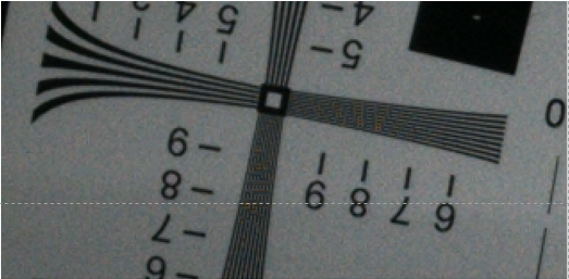
Figure 4-12: Misjudgement of Direction at High-Frequency Region

4.1.4.2. Adjustment Interface

Select BayerCompensation from the menu on the left-hand side. You will find the DeMosaic interface to the right of your screen.

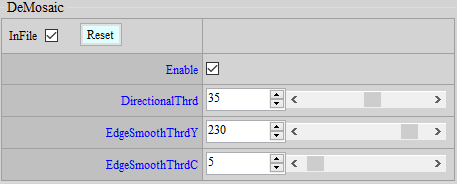
Figure 4-13: DeMosaic Adjustment Interface

4.1.4.3. Parameter Description

DirectionalThrd : Directional or non-directional interpolation threshold. Parameter range: 0 ~ 63. The larger the value is, the more details will become blurred.

EdgeSmoothThrdY : Smoothing by brightness. Parameter range: 0 ~ 255. The smaller the value, the less sharp the edge, and the less likely for artifacts to appear.

EdgeSmoothThrdC : Smoothing by saturation. Parameter range: 0 ~ 127. The smaller the value, the less sharp the edge, and the less likely for artifacts to appear.

4.2. DynamicDP & NRDespike Adjustment¶

As described in the preceding section, peak noise is basically regarded as a special noise, and hence needs to be removed or weakened by a specific function.

It is recommended that peak noise be handled before normal noise so as to avoid impairing the image quality when using other denoise functions to deal with peak noise. Two functions — DynamicDP and NRSpikeNR — are available for coping with peak noise. Both functions can be used simultaneously.

4.2.1. DynamicDP (Dynamic Defective Pixel Correction)¶

DPC handles peak noise by replacing it, and is hence more visible in effect.

4.2.1.1. Adjustment Interface

Select “BayerCompensation” from the menu on the left-hand side. You will find the DynamicDP interface to the right of your screen.

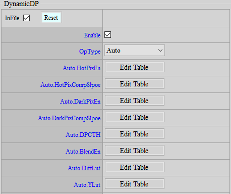
Figure 4-14: DynamicDP Adjustment Interface

4.2.1.2. Parameter Description

HotPixEn : Hot pixel peak enable.

HotPixCompSlope : Threshold to determine if a pixel is a hot pixel peak. Parameter range: 0 ~ 255. The greater the value is, the more difficult it is to be judged as a hot pixel peak, and vice versa.

DarkPixEn : Dark pixel enable.

DarkPixCompSlope : Threshold to determine if a pixel is a dark pixel peak. Parameter range: 0 ~ 255. The greater the value is, the more difficult it is to be judged as a dark pixel peak, and vice versa.

DPCTH : Same-channel pixel threshold. Parameter range: 0 ~ 255. The greater the value is, the more unlikely it will be treated as a defective pixel, and vice versa.

BlendEn : Blending enable.

DiffLut : Blending depends on the difference between DPC result and original one. Parameter range: 0 ~ 1024. The greater the value is, the more likely it will be replaced by DPC result.

YLut : Blending depends on Y. Parameter range: 0 ~ 1024. The greater the value is, the more likely it will be replaced by DPC result.

4.2.1.3. Adjustment Steps

Determine to enable HotPix or DarkPix.
DPCTH is used to determine same-channel pixel difference. Only when DPCTH and PixCompSlope are both established will defective pixel compensation be performed.
Increase PixCompSlope gradually until peak noise and details reach an acceptable balance.
Enable BlendEn, tuning DiffLut and YLut to balance peak noise and details.

4.2.2. DynamicDP Cluster¶

DynamicDP detects defect by the difference between the present point and its neighboring points. DynamicDP cluster takes into account the possibility of the neighboring points being defective too, and so will exclude the neighboring brightest or darkest points first.

4.2.2.1. Adjustment Interface

Select “BayerCompensation” from the menu on the left-hand side. You will find the DynamicDP_Cluster interface to the right of your screen.

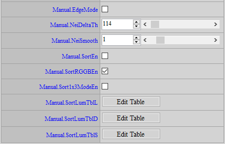
Figure 4-15: DynamicDP_Cluster Adjustment Interface

4.2.2.2. Parameter Description

EdgeMode : Edge mode enable. It removes 0 ~ 1 brightest or darkest point.

NeiDeltaTh : Threshold values of difference between 8 neighboring points and the average value of these 8 points. If Diff > threshold, then the total number (count) is calculated.

NeiSmooth : Accumulative threshold. If the count is smaller than the threshold, the brightest or darkest point will be replaced.

SortEn : Sort mode enable. Sort the neighboring points in order to screen out the brightest (darkest) point that meets the following conditions — the difference between the brightest (darkest) point and the second brightest (darkest) point is large enough, and the difference between the second brightest (darkest) point and the third brightest (darkest) point is small enough. It means that only one point around is very bright (dark), and the other points are of similar brightness (darkness), and so we can replace that one bright (dark) point. The maximum number of compensations is removing 0 ~ 2 brightest point and 0 ~ 1 darkest point.

SortRGGBEn : Sort mode channel enable.

Sort1x3ModeEn : 1x3 mode enable. If the two points around the center point happen to be the brightest and the second brightest points, and the difference between the second brightest point and the third brightest point is larger than SortLumaTblL, the two brightest points will be replaced by the third brightest point.

SortLumaTblL : Threshold values of the two brightest points, which can be tuned by lumimance. If larger than this threshold, replacement will take place. A larger value means that the brightest point need to be much brighter than the second brightest point to be replaced by the second brightest point, which means that the judgment conditions are stricter.

SortLumaTblD : Threshold values of the two darkest points, which can be tuned by lumimance. If larger than this threshold, replacement will take place. A larger value means that the darkest point need to be much darker than the second darkest point to be replaced by the second darkest point, which means that the judgment conditions are stricter.

SortLumaTblS : Threshold values of the second and third brightest (darkest) points, which can be tuned by lumimance. If smaller than this threshold, replacement will take place. A smaller value means that the second and third brightest (darkest) points must be more similar to replace the brightest (darkest) point, which means that the judgment conditions are stricter.

4.2.2.3. Adjustment Steps

If the defect cannot be detected by DynamicDP, try to enable EdgeMode or SortEn. The larger the strength, the more defects would be detected. However, more details will be lost.
It is suggested to make DynamicDP_Cluster setting more relaxed to detect more defects, and do blending by the defect level.

4.2.3. NRDeSpike¶

NRDeSpike handles peak noise by drawing the pixel of concern near the median of the neighboring pixel, and is therefore capable only of weakening, and not eliminating, the peak noise.

4.2.3.1. Adjustment Interface

Select BayerDenoise from the menu on the left-hand side. You will find the NRDeSpike interface to the right of your screen.

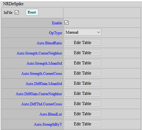
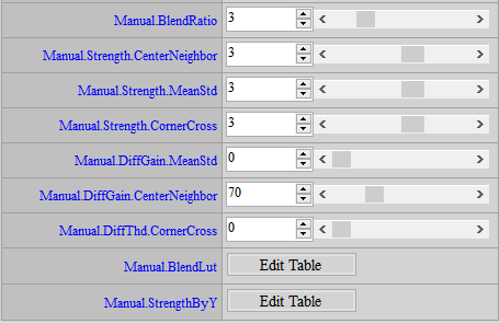
Figure 4-16: NRDeSpike Adjustment Interface

4.2.3.2. Parameter Description

NRDeSpike employs the following three methods simultaneously to determine the despike strength. The weakest one will be taken as the final strength.

< CenterNeighbor >

Strength : Strength based on CenterNeighbor. Parameter range: 0 ~ 5. The greater the value, the greater the strength.

DiffGain : Threshold based on CenterNeighbor. DeSpike strength will be set to the strongest if the value is greater than this threshold. Parameter range: 0 ~ 255. The smaller the value is, the easier it is to apply the strongest despike strength.

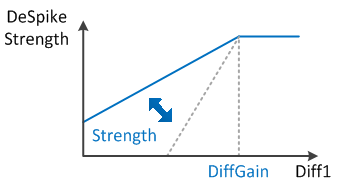
Figure 4-17: CenterNeighbor Parameters
< CornerCross >

Strength : Strength based on CornerCross. Parameter range: 0 ~ 5. The greater the value, the greater the strength.

DiffThd : Threshold based on CornerCross. Despike strength will be set to the strongest if the value is smaller than this threshold. Parameter range: 0 ~ 255. The greater the value is, the easier it is to apply the strongest despike strength.

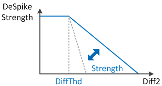
Figure 4-18: CornerCross Parameters
< MeanStd >

Strength : Strength based on MeanStd. Parameter range: 0 ~ 5. The greater the value, the greater the strength.

DiffGain : Gain value of one of the MeanStd analyzing conditions. Parameter range: 0 ~ 31. The greater the value is, the easier it is to apply the strongest despike strength.

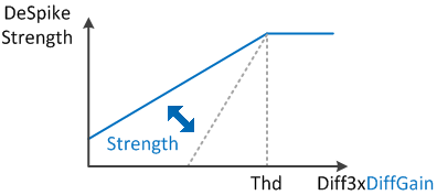
Figure 4-19: MeanStd Parameters

BlendRatio : Overall strength setting. Parameter range: 0 ~ 15. The greater the value is, the less obvious the peak will be.

BlendLut : Median/mean mixing ratio selection. Parameter range: 0 ~ 2047. The horizontal axis represents the difference between the center and the neighborhood, the largest difference falling at the rightmost end. The vertical axis represents the mixing ratio. A larger value will tend toward median method, and a smaller value, toward mean method.

StrengthByY : Applies different strength based on different brightness. Parameter range: 0 ~ 127. 64 means no change. The smaller the value, the weaker the strength; the greater the value, the stronger the strength.

4.2.3.3. Adjustment Steps

Since the weakest strength among the three methods will be used as the final strength, adjusting one single parameter may not necessarily arrive at an expected effect, and so we suggest following the steps below to achieve the best possible adjustment.

Set BlendRatio to 15, to ease your inspection.
Find out the optimal parameters for each method. Set the strength of the other two to the strongest when adjusting one of the three methods.

\< Taking CenterNeighbor as an example >
1. Set CornerCross and MeanStd to the maximum value.
  
  Strength.CornerCross=5
  
  DiffThd.CornerCross=255
  
  Strength.MeanStd=5
  
  DiffGain.MeanStd =31
2. Set Strength.CenterNeighbor to 0, and decrease DiffGain.CenterNeighbor from 255 gradually until peak noise and detail come to an acceptable extent.
3. Record the adjusted parameters.
Adjust the parameters of the other two methods with reference to step 2. When done, copy the parameter values onto the corresponding fields on the tool interface.
Decrease BlendRatio gradually until peak noise and detail come to an acceptable extent.
Since spike and DPC share same source input, defective pixel can be mixed into the spike compensation result. In this case, you can adjust BlendLut to have the spike result tend toward median method to exclude the defective pixel. If no such problem occurs, you can apply the mean method to obtain a smoother result.

4.3. NR3D, NRLuma & NRChroma Adjustment¶

NR3D is a very powerful function. Apart from decreasing temporal noise, NR3D can also adjust the strength of NRLuma and Sharpness against static and/or dynamic areas. Hence, it is suggested that you start with NR3D, and apply NRChroma later, if necessary.

4.3.1. NR3D ON¶

NR3D is primarily used for reduction of temporal noise including Y and color noise. Stronger NR3D can effectively reduce noise, but there’s the side effect of creating ghost images. Therefore, we suggest that you adjust to a point where noise and ghost images find an acceptable balance.

4.3.1.1. Adjustment Interface

Select Denoise from the menu on the left-hand side. You will find the NR3D interface to the right of your screen.

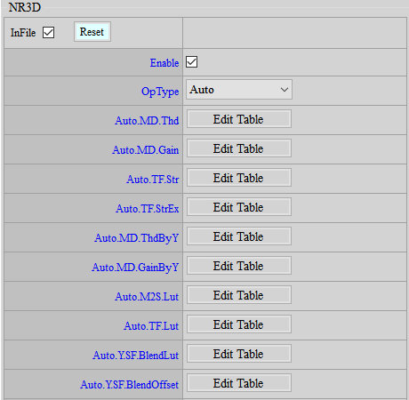
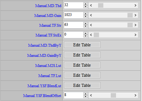
Figure 4-20: NR3D Adjustment Interface

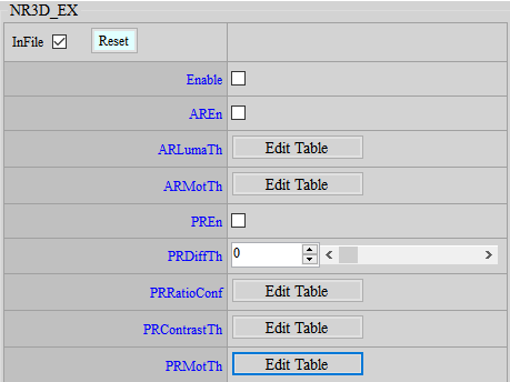
Figure 4-21: NR3D_EX Adjustment Interface

4.3.1.2. Parameter Description

< Spatial Domain Denoise, SF series parameters>

For details on the parameter control, please refer to NRLuma, NRLuma_Adv, NRChroma, and NRChroma_Adv.
< Temporal Domain Denoise, MD, TF series parameters >

TF.LUT : mainly utilizes difference and motion information to decide the temporal denoise strength. If difference and motion are small, it is very likely the area is a static area; otherwise, a dynamic one. Parameter range: 0 ~ 4095.

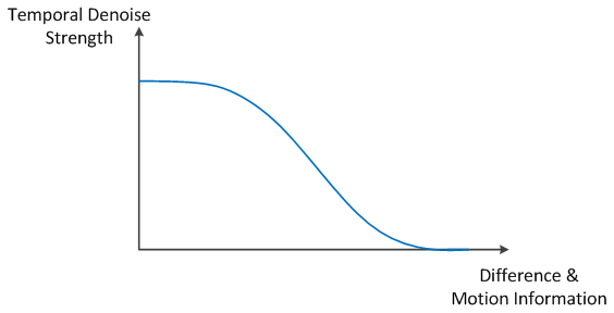
Figure 4-22: TF.LUT

MD.Thd : Motion threshold control. Parameter range: 0 ~ 255. The larger the value, the stronger the NR3D function. Areas with motion lower than the threshold value will be judged as static areas. We suggest that this parameter be set to a value not greater than 10.

MD.Gain : Motion scale control. Parameter range: 0 ~ 10230. The larger the value and the smaller the motion information, the stronger the NR3D function.

MD.ThdByY : Motion threshold value based on brightness. Parameter range: 0 ~ 255. The larger the value, the stronger the NR3D function.

MD.GainByY : Motion scale based on brightness. Parameter range: 0 ~ 255. The larger the value and the smaller the motion information, the stronger the NR3D function. This can be increased against noise with greater brightness, or decreased against noise with brightness having indeterminable ghost images.

TF.Str : NR3D strength. Parameter range: 0 ~ 64. The larger the value, the stronger the NR3D function is.

TF.StrEx : Extra NR3D strength. Parameter range: 0 ~ 64. The larger the value, the stronger the NR3D function is.

M2S.LUT : NR3D strength control for the transition from static area to dynamic area. Parameter range: 0 ~ 31. The larger the value, the weaker the NR3D function and the stronger the NRLuma function. The dynamic-to-static curve should not be too steep; otherwise, the moving object and the intermediate zone that transitions to the static area would appear unnatural.
< Denoise by motion series parameters>

Y.SF.BlendLUT : Adjust NRLuma strength based on motion information. Parameter range: 0 ~ 16. Dynamic on the left and static on the right. The larger the value, the stronger the NRLuma strength.

Y.SF.BlendOffset : Control the extent of NR3D compensation to be written back to the NR3D reference frame motion information. Parameter range: 0 ~ 16. The larger the value, the higher the NR3D compensation ratio.
< NR3D Alpha Blending Refine series parameters >

AREn : Switch to turn on/off the NR3D strength limit based on brightness and motion information. Parameter range: 0 ~ 1.

ARLumaTh : When Luma \< LumaTh[0], the NR3D strength remains unchanged; when Luma > LumaTh[1], the NR3D strength is 0. Parameter range: 0 ~ 255.

ARMotTh : When motion \< MotTh[0], the NR3D strength remains unchanged; when motion > MotTh[1], the NR3D strength is 0. Parameter range: 0 ~ 255.
< NR3D Purple False Color Compensation series parameters >

In cases where screen rotation is used, you can enable this function to help NR3D to more accurately discern the motion surrounding purple fringe, lest any such motion is misjudged as dynamic, thereby leading to NR3D stability issue. DiffTh, RatioConf and ContrastTh will be used to determine the extent of purple fringe. If the three conditions all recognize the motion as purple fringe, the motion adjacent to the purple fringe can be re-distributed to be more static.

PREn : Motion switch to assist NR3D in the judgement of purple fringe.

PRDiffTh : According to the PFC result, purple fringe will be confirmed if PFC compensation > PRDiffTh. Parameter range: 0 ~ 4095. The smaller the value is, the more likely an area will be recognized as purple fringe.

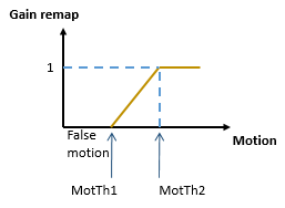
PRRatioConf : To determine if the color concerned is similar to the purple fringe. Parameter range: 0 ~ 16. The horizontal axis represents color resemblance. The closer to the right side of the horizontal axis, the more resemblance to purple fringe. The vertical axis represents purple fringe judment criterion. The larger the value, the more likely an area will be recognized as a purple fringe.

PRContrastTh : Parameter to judge the extent of contrast. When the contrast is high, purple fringe is more likely to occur. Parameter range: 0 ~ 16. If the contrast is smaller than ContrastTh1, the area will not be treated, and if the contrast is larger than ContrastTh2, the area will be regarded as a purple fringe.

PRMotTh : If the purple fringing possibility is high, the motion information will be re-defined using the following measure. Set MotTh1 to exclude motion information below this threshold as misjudged case, and re-distribute the motion as 0, which means static. For motion information above MotTh2, which means normal motion, nothing will be done. On the other hand, if purple frnge is not found, the motion information will remain unchanged too.

4.3.1.3. Adjustment Steps

First, adjust the NR3D strength with respect to still images, to reduce dynamic image noise level.
- Adust NR3D strength, to make the picture look stable as a whole. We suggest that you set TF.Str to 63, and increase MD.Gain to a degree where the picture appears stable. If it takes a very high MD.Gain value to make the picture stable, you can increase MD.Thd in the meantime, but the value should preferably be no greater than 10.
Second, adjust the NR3D strength against the area after object movement.
- Adjust M2S.LUT. The M2S.LUT curve should not be too steep; otherwise, the transition of the area after object movement from blurred to clear will leave a visible and unnatural borderline.
- You can fine-tune the value based on the suggested setting. If fewer residual images are preferred, you can set to a greater value, so that the NRLuma for the area after object movement will get stronger and last longer, but the weaker NR3D will appear unstable; on the other hand, if you prefer to have the area after object movement clearer, and a few residual images are acceptable, you can set to a smaller value to mitigate the unstable issue, but particle noise might occur.
- Suggested setting: {24, 18, 11, 8, 7, 7, 6, 6, 6, 5, 5, 5, 5, 4, 4, 4}
Fine-tune for balance between motion blur and noise level.
- Adjust Y.SF.BlendLUT, where the dynamic area is located on the left-hand side and the static area the right-hand side. Adjust up the value gradually until both motion blur and noise level are acceptable. The value of the last cell should preferably be fixed at 0, so as to maintain the detail of the still image. It is advisable to use this function in combination with NRLuma BlendRatio and FilterLevel.
- For noise generated after motion, apart from adjusting NR2D strength based on the motion information, you can also adjust Y.SF.BlendOffset to do some NR3D compensation in response to the motion, to reduce the noise. Because this will be updated only to the NR3D reference frame, no impact will be brought onto the image.
For brightness with apparent ghost image phenomenon, adjust down MD.GainByY against the corresponding bright area, to an extent both ghost images and noise are acceptable.
With higher gain, NRLuma alone is not enough to reduce motion noise. In such cases, you can modify TF.LUT to slow down the curve and to thereby increase the NR3D strength of motion area, noting, however, that the ghost image problem can become worse. If you set the value of the last cell to a non-zero value, pink ghost image will appear at the edge of moving objects. In this case, you can use AREn to limit the NR3D strength against brighter, fast-moving area to eliminate such ghost images.
NR3D has an additional mechanism which enables the results from the NR3D process to come closer to the results from the current frame. Yet, this mechanism might also cause disturbance upon the NR3D results. You may use “Dummy_Ex/Dummy1” to prevent such issue when additional adjustment is required. Please refer to Chapter 6 for a detailed introduction on Dummy_Ex.
Two different modes for motion information transmission are available. Additional adjustments can be made by using “Dummy_Ex/Dummy1.” Please refer to Chapter 6 for a detailed introduction on Dummy_Ex.

4.3.2. NR3D OFF¶

In cases where DRAM is not installed for purpose of cost reduction, NR3D will not be available. Set forth below are the steps to achieve the denoise in the absence of NR3D.

4.3.2.1. Adjustment Interface

Please refer to Section 4.3.1.1.

4.3.2.2. Parameter Description

Please refer to Section 4.3.1.2.

4.3.2.3. Adjustment Steps

Be sure that the Iqfile is an NR3D-Off version.

In the NR3D interface, only spatial domain series parameters can be adjusted, including Y.SF.STR.

For NRLuma, we suggest setting Wei to 63 (maximum value) to adjust LumaX and LumaStrengthByY.

The adjustment steps for despike are the same as those in the case of NR3D on.

If you have further fine-tuning requirement, denoise against the remaining portions can be done, using the same adjustment steps as those used for NR3D on.

4.3.3. NRLuma¶

4.3.3.1. Adjustment Interface

Select Denoise from the menu on the left-hand side. You will find the NRLuma interface to the right of your screen.

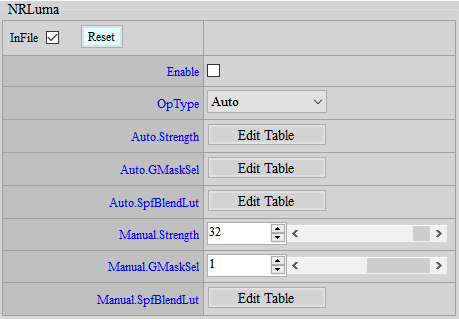
Figure 4-23: NRLuma Adjustment Interface

4.3.3.2. Parameter Description

Strength : NRLuma final strength control. Parameter range: 0 ~ 63. The larger the value, the higher the strength.

GMaskSel : Gaussian Filter size selection. Parameter range: 0 ~ 1. 0 for smaller size, and 1 for bigger size.

SpfBlendLut : Uses Gaussian Filter (SPF) and bilateral filter for blending. If the center pixel is similar to the neighboring pixels, you can apply more Gaussian filter results for smoother effect; if dissimilar, you can apply Biliteral filter results to maintain detail. The horizontal axis represents the degree of similarity. The closer to the right side, the higher similarity. The vertical axis represents Gaussian blending strength; parameter range: 0 ~ 256. The larger the value, the higher blending strength. You might use Dummy/Dummy1 to adjust the intensity of bilateral filter. Please refer to Chapter 6 for a detailed introduction on Dummy_Ex.

4.3.3.3. Adjustment Steps

The spatial denoise strength should have been adjusted to a suitable value during NR3D adjustment. If further adjustment is required, use NRLuma for fine-tuning.

Tuning SpfBlendLut to balance noise reduction and detail retention.

4.3.4. NRLuma_Adv¶

4.3.4.1. Adjustment Interface

Select Denoise from the menu on the left-hand side. You will find the NRLuma_Adv interface to the right of your screen.

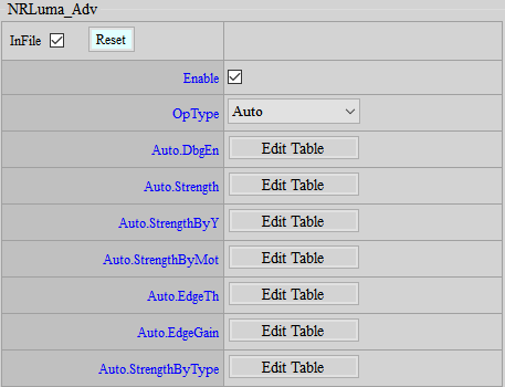
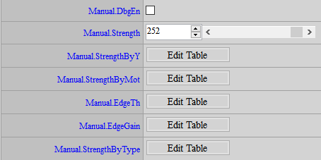
Figure 4-24: NRLuma_Adv Adjustment Interface

4.3.4.2. Parameter Description

DbgEn : Shows the edge strength detected by NRLuma_Adv.

Strength : NRLuma_Adv final strength control. Parameter range: 0 ~ 255. The larger the value, the higher the strength.

StrengthByY : Applies different NR strength against different brightness. The closer to the right side of the horizontal axis, the higher the brightness. Parameter range: 0 ~ 32. The larger the value, the higher the strength. Default value is 0, which means no strength adjustment, and so only increase of strength is available.

StrengthByMot : Applies different NR strength against different motion. The closer to the right side of the horizontal axis, the smaller the motion. Parameter range: 0 ~ 32. The larger the value, the higher the strength. Default value is 0, which means no strength adjustment, and so only increase of motion is available.

EdgeTh : Threshold for edge judgement. The closer to the right side of the horizontal axis, the higher the brightness. When the edge is smaller than this threshold, it is regarded as noise, and will be treated using NR function. When the edge is larger than this threshold, it is confirmed as an edge. The stronger the edge, the weaker the NR effect. Parameter range: 0 ~ 16383. The larger the value, the less likely an edge is to be recognized as an edge.

EdgeGain : Edge control parameter. The closer to the right side of the horizontal axis, the higher the brightness. Edge higher than this threshold will be subjected to strength control. The stronger the edge, the weaker the NR effect. Parameter range: 0 ~ 65535. The larger the value, the higher the strength.

StrengthByType : There are two filter types for NR. StrengthByType [0] is a filter strength retaining more detail, while StrengthByType [1] is a filter strength with better denoise effect but worser detail retainability. Filter blending of these two filters is done depending on edge strength. The larger the value, the stronger the NR effect.

4.3.4.3. Adjustment Steps

The main purpose is to fine-tune the NR3D and NRLuma result.

Adjust EdgeTh and EdgeGain, to determine which area is the edge area.
Set StrengthByY and ByMot to 0, and adjust StrengthByType, to apply different NR strength to edge area and non-edge area.
Strengthen NR depending on different brightness and motion.

4.3.5. NRChroma¶

NRChroma is used to suppress the color noise on screen.

4.3.5.1. Adjustment Interface

Select Denoise from the menu on the left-hand side. You will find the NRChroma interface to the right of your screen.

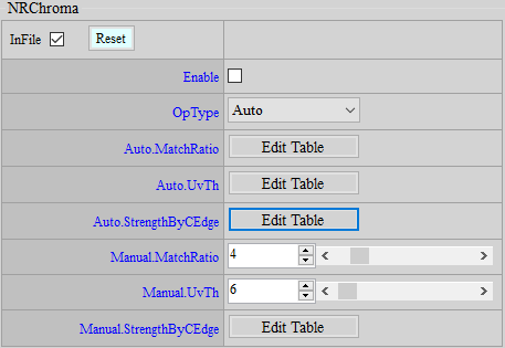
Figure 4-25: NRChroma Adjustment Interface

4.3.5.2. Parameter Description

MatchRatio : Threshold value of fitting ratio. Parameter range: 0 ~ 31. The larger the value, the greater the strength.

UvTh : U/V noise threshold value. Parameter range: 0 ~ 256. The larger the value, the greater the strength.

StrengthByCEdge : Controls NRChroma strength by color edge. Parameter range: 0 ~ 511. The larger the value, the greater the strength.

4.3.5.3. Adjustment Steps

Tune MatchRatio and UvTh to make color noise scattered. Too strong values will lead to color bleeding, so tune to an acceptable extent.
Lower the StrengthByCEdge to further restrain the color-bleeding area.

4.3.6. NRChroma_Adv¶

NRChroma_Adv is used to suppress the color noise on screen.

4.3.6.1. Adjustment Interface

Select Denoise from the menu on the left-hand side. You will find the NRChroma_Adv interface to the right of your screen.

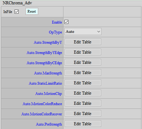
Figure 4-26: NRChroma_Adv Adjustment Interface

4.3.6.2. Parameter Description

StrengthByY : Applies control of different NR strength against different brightness. The closer to the right side of the horizontal axis, the higher the brightness. Parameter range: 0 ~ 255. The larger the value, the higher the strength.

StrengthByYEdge : Applies control of different NR strength against different edge using Luma to detect the size of the edge. The closer to the right side of the horizontal axis, the bigger the edge. Parameter range: 0 ~ 63. The larger the value, the higher the strength.

StrengthByCEdge : Applies control of different NR strength against different edge using Chroma to detect the size of the edge. The closer to the right side of the horizontal axis, the bigger the edge. Parameter range: 0 ~ 255. The larger the value, the higher the strength.

MaxStrength : Controls NR strength against area with small Y/C difference. Parameter range: 0 ~ 255. The larger the value, the higher the strength.

StaticLimitRatio : Controls NR strength against static area. Parameter range: 0 ~ 63. The larger the value, the higher the strength.

MotionClip : Provides more NR strength against motion area. Parameter range: 0 ~ 255. The larger the value, the higher the strength.

MotionColorReduce : Reduces the extent of saturation against motion area. Parameter range: 0 ~ 255. The larger the value, the more the saturation is reduced.

MotionColorRecover : Recovers the extent of saturation of the motion area reduced by MotionColorReduce by gain. Parameter range: 0 ~ 255. The larger the value, the more the saturation is recovered.

PreStrength : Performs simple denoise function against chroma. Parameter range: 0 ~ 128. The larger the value, the higher the strength.

4.3.6.3. Adjustment Steps

Set MotionClip to 0.
Observe the static area and adjust MaxStrength and StaticLimitRatio, to tune NR to the extent that color noise is acceptable.
Observe the dynamic area and adjust MotionClip to strengthen the moving portion based on the NR strength in step 1. If the tuning by MotionClip is not strong enough, go back to step 1 to increase the strength.
Where necessary, adjust MotionColorReduce to suppress the saturation of the moving portion. This will help NRChroma_Adv to more easily remove color noise. If decrease in moving portion of saturation is not desired, adjust MotionColorRecover to recover the saturation of the moving portion.

4.4. Sharpness Adjustment¶

The adjustment of Y.PK LUT in NR3D is mainly to allow dynamic area and static area to have a suitable sharpness strength of their own. The adjustment of sharpness strength based on other conditions is, on the other hand, done by Sharpness, which include, for example, sharpness strength determined by different brightness, sharpness strength based on center of picture, and sharpness strength controlled by black or white edge.

4.4.1. Sharpness¶

4.4.1.1. Adjustment Interface

Select Sharpness from the menu on the left-hand side. You will find the Sharpness interface to the right of your screen.

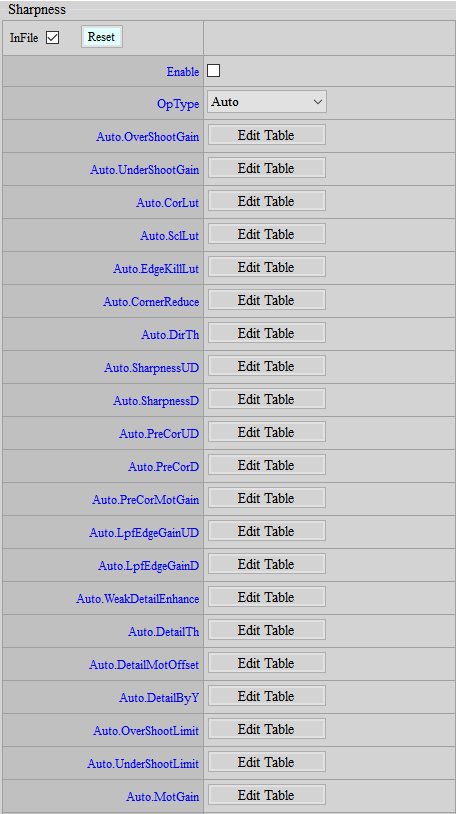
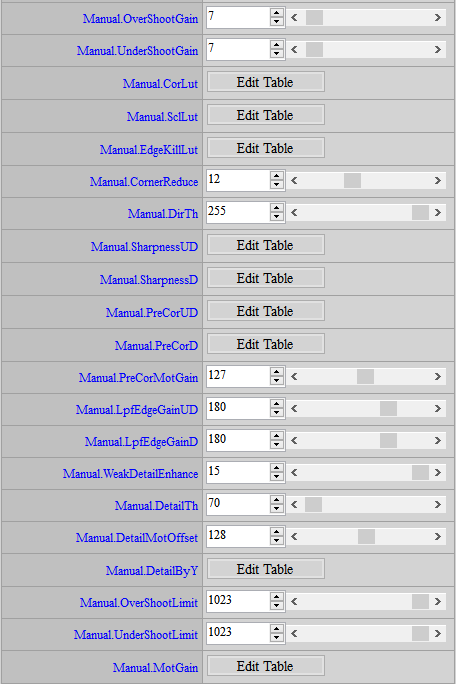
Figure 4-27: Sharpness Adjustment Interface

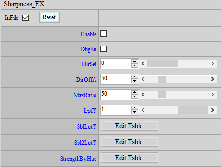
Figure 4-28: Sharpnes_EX Adjustment Interface

4.4.1.2. Parameter Description

OverShootGain : Adjustment of strength against white edge. Parameter range: 0 ~ 255. The greater the value, the stronger the strength.

UnderShootGain : Adjustment of strength against black edge. Parameter range: 0 ~ 255. The greater the value, the stronger the strength.

The two parameters, if set to too great a value, can lead to an increase of noise. In this case, you can utilize CorLut to suppress the level of noise caused by OverShootGain and UnderShootGain, at the expense of detail retention, however.

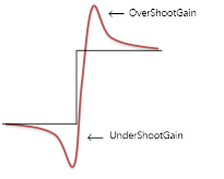
Figure 4-29: OverShootGain & UnderShootGain

CorLut : Adjusts edge output based on brightness. Parameter range: 0 ~ 255. The greater the value, the weaker the edge.

SclLut : Adjusts edge output based on brightness. Parameter range: 0 ~ 255. The greater the value, the stronger the edge.

EdgeKillLut : There are 0 ~ 255 portions depending on the strength of edge. Six nodes are available to adjust the output size of the edge. It is recommended that the first cell be 0 to prevent noise from being enhanced at edge. Parameter range: 0 ~ 1023. The greater the value, the stronger the edge. If you find node distribution on the horizontal axis inadequate, use Dummy_Ex/Dummy0 for further adjustment. Please refer to Chapter 6 for a detailed introduction on Dummy_Ex.

CornerReduce : The farther the pixel is from the image center, the smaller the sharpness effect will be. The more peripheral the lens, the worse the image quality. Reducing sharpness effect can improve sharpness strength of the edge noise set at the fartherest corner. Parameter range: 0 ~ 32. The strength of the center will remain unchanged, while the strength of the center-to-corner area will be determined by interpolation.

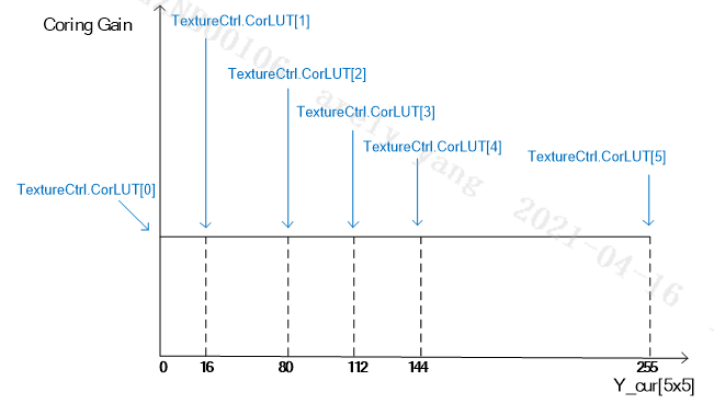
Figure 4-30: extureCtrl.CorLUT

Figure 4-31: SclLUT

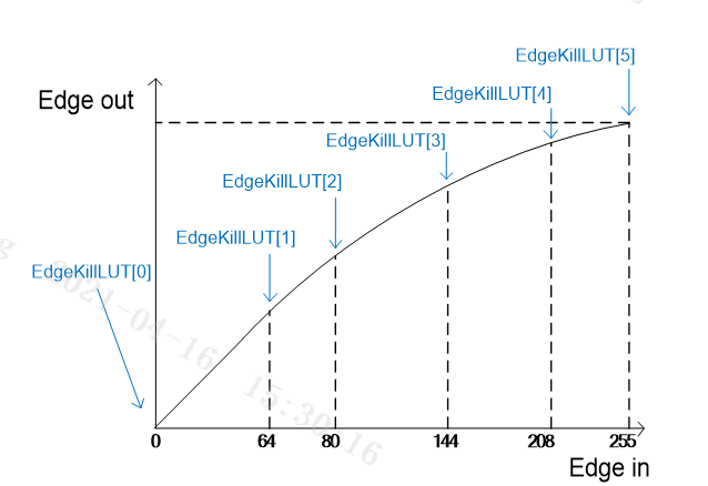
Figure 4-32 EdgeCtrl.OverShootGain & EdgeCtrl.UnderShootGain

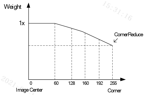
Figure 4-33 CornerReduce

DirTh : Threshold for determining direction. If this threshold is exceeded, a directional filter for edge enhancement will be used. This has the merit of a continual edge, but the edge of small details will be enhanced, causing the image to look unnatural.

SharpnessUD : For enhancing non-directional detail texture. This can be used to enhance sharpness of small texture, such as hair and sod. SharpnessUD[0] can be used for high-frequency case, and SharpnessUD[1] for low-frequency case. Parameter range: 0 ~ 1023. The greater the value, the stronger the edge.

SharpnessD : For enhancing sharpness along the direction of the edge to strengthen image edge as a whole. Note that the edge will appear jaggy if over-enhanced. SharpnessD[0] can be used for high-frequency case, and SharpnessD[1] for low-frequency case. Parameter range: 0 ~ 1023. The greater the value, the stronger the edge.

PreCorUD : Performs coring against non-directional edges. PreCorUD[0] can be used for high-frequency case, and PreCorUD[1] for low-frequency case. Parameter range: 0 ~ 63. The greater the value, the weaker the edge.

PreCorD : Performs coring against directional edges. PreCorD[0] can be used for high-frequency case, and PreCorD[1] for low-frequency case. Parameter range: 0 ~ 63. The greater the value, the weaker the edge.

PreCorMotGain : Enhances coring against a motion area based on the settings of PreCorUD and PreCorD. Parameter range: 0 ~ 255. The greater the value, the weaker the edge within the motion area.

LpfEdgeGainUD : Controls edge gain by a configurable non-directional high-frequency/low-frequency output ratio based on the SharpnessUD, PreCorUD, and PreCorMotGain results. Parameter range: 0 ~ 255. The bigger the value, the higher the low-frequency strength and the weaker the high-frequency strength. The smaller the value, the weaker the low-frequency strength and the higher the high-frequency strength.

LpfEdgeGainD : Controls edge gain by a configurable directional high-frequency/low-frequency output ratio based on the SharpnessD, PreCorD, and PreCorMotGain results. Parameter range: 0 ~ 255. The bigger the value, the higher the low-frequency strength and the weaker the high-frequency strength. The smaller the value, the weaker the low-frequency strength and the higher the high-frequency strength.

WeakDetailEnhance : Enhances edge against textile with weak details. Parameter range: 0 ~ 255. The greater the value, the stronger the edge.

DetailTh : SharpnessUD threshold, can be used to lower the edge at flat area.

DetailMotOffset : Adjusts SharpnessUD by the extent of motion. In case that motion distribution is not very satisfactory, use Dummy/Dummy2 for further adjustment. Please refer to Chapter 6 for a detailed introduction.

DetailByY : Adjusts SharpnessUD by Y.

OverShootLimit : Edge adjustment depending on the brightest point in the neighberhood. Zero value means the max. edge equals to the Y value of the brightest point in the neighberhood, namely, no overshoot edge.

UnderShootLimit : Edge adjustment depending on the darkest point in the neighberhood. Zero value means the min. edge equals to the Y value of the darkest point in the neighberhood, namely, no undershoot edge.

Figure 4-34: OverShootLimit & UnderShootLimt

MotionGain : Adjusts the final edge based on the extent of motion. The horizontal axis represents the extent of motion. The closer to the right side, the stiller. Parameter range: 0 ~ 255. The greater the value, the stronger the edge. Value 128 means no change.

\< Sharpness_EX>

DbgEn : Debug mode, in which only edge to be compensated will be shown on screen.

DirSel : Directional judgement of SharpnessD. When set to 0, the maximum value of all directions represent the direction to be used, and 1 means determining the direction based on a simple anti-noise measure.

DirOffA : The blending ratio of SharpnessD and SharpnessUD is determined by the strength of the direction. To enhance the output of SharpnessUD, you can use the parameter DirOffA. Parameter range: 0 ~ 255. The greater the value, the stronger the non-directional edge.

MaxRatio : If the segments are discontinuous, adjust DirTh first. And if this does not help, adjust up this parameter then. Parameter range: 0 ~ 255. The greater the value, the stronger the edge.

LpfY : Performs LPF process against the horizontal axis Y of CorLut and SclLut, to avoid using different Cor and Scl results due to motion of noise. 0 means LPF disabled, and 1 means LPF enabled.

SblLutY : The strength of the low-frequency part of SharpnessD will be determined using Sobel filter. This parameter can adjust the strength by Y. The horizontal axis represents brightness. The closer to the right side, the brighter. Parameter range: 0 ~ 255. The greater the value, the bigger the strength.

Sbl2LutY : The strength of the high-frequency part of SharpnessD will be determined using Sobel filter. This parameter can adjust the strength by Y. The horizontal axis represents the level of brightness. The closer to the right side, the brighter. Parameter range: 0 ~ 255. The greater the value, the bigger the strength.

StrengthByHue : Adjusts sharpness by hue. Edge sharpness can be increased or decreased against a specific hue. The horizontal axis represents hue. You have 24 even parts for degrees 0 to 360 to choose from. The greater the value, the stronger the edge. 64 means no adjustment is done.

4.4.1.3. Adjustment Steps

If you follow the recommendation set forth above, the initial Sharpness parameters should have the following values:

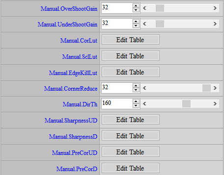
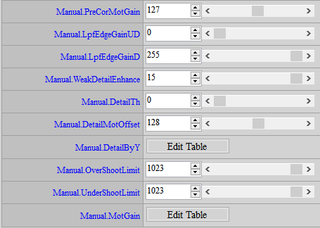
Figure 4-35: Sharpness Suggested Default Value

Observe the area with strong edge. Then adjust the OverShootGain and UnderShootGain until black/white edge enhancement is acceptable.
Adjust DirTh. Do not have the continuous segments go beyond the edge in the UD direction, lest the segments should become discontinuous.
Observe the flat area to see if any noise has been enhanced by sharpness. If yes, increase the PreCorUD and PreCorD of high-frequency and low-frequency to exclude that area. Note, however, that a greater value means more edge cannot be enhanced, and that, as a consequence, the picture will get more blurry. Hence, while adjusting, see if any spot requiring edge enhancement has been omitted. If noise variation is not easily detectable, adjust up the OverShootGain and UnderShootGain to an excessive degree to facilitate coring adjustment. By so doing, it would not be necessary to 100% remove the noise, since some of the noise will be unperceivable once the OverShootGain and UnderShootGain are set back to their normal values. Suppressing the node previous to Edge LUT can arrive at a similar effect, too, but the adjustment is relatively more difficult and is therefore not suggested, unless you are very familiar with Edge LUT.
Observe the dark area to see if any noise is enhanced by sharpness. If yes, adjust up SclLut gradually to suppress the sharpness, and therefore the noise, of the dark area.
Observe the image corner and see if any noise is increased due to ALSC compensation. If yes, adjust down CornerReduce to reduce the sharpness strength of the corner.
Adjust SharpnessUD and SharpnessD to enhance directional and non-directional detail, then enlarge DetailTh to avoid applying overly large SharpnessUD in flat area. If necessary, adjust DetailByY for fine-tuning.
If necessary, adjust OverShootLimit and UnderShootLimit to limit overshoot or undershoot edge.

5. WDR¶

Wide Dynamic Range (WDR) is a technology used to expand the range of dynamic area, thereby allowing details of bright pixels and dark pixels to co-exist in the same image with distinctiveness.

5.1. WDR¶

The WDR, a local WDR in nature, helps ehance image dynamic range locally and is recommended for WDR adjustment.

5.1.1. Adjustment Interface¶

Select WDR from the menu on the left-hand side. You will find the WDR interface to the right of your screen.

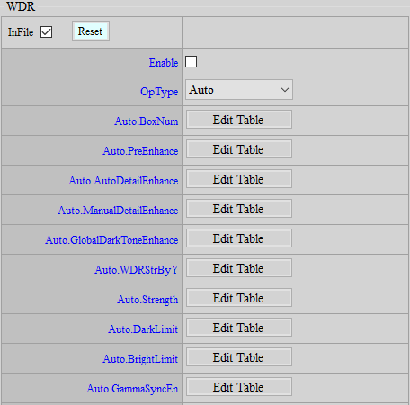
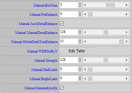
Figure 5-1: WDR Adjustment Interface

5.1.2. Parameter Description¶

BoxNum : 2 ~ 4 size options available for different sensor aspect ratios. Can be adjusted according to the size of the object to be highlighted. The greater the BoxNum, the smaller the Box and the more suitable it is for object of smaller size. It cannot vary by ISO.

PreEnhance : Bright area dynamic interval ratio. The greater the value, the bigger the dynamic interval alloted to the bright area; the smaller the value, the bigger the dynamic interval alloted to the dark area. Parameter range: 1 ~ 6, default is 2. Additionally, values 11 ~ 15 are added based on the default value. The greater the value, the brighter, yet the vaguer, the dark area. This parameter cannot vary by ISO. Besides, it will not work when GammaSyncEn=1.

AutoDetailEnhance : Additional detail enhancement for bright pixels or dark pixels. 1: Auto; 0: Manual.

ManualDetailEnhance : When AutoDetailEnhance is 0, you can manually control the extent of detail enhancement to be exerted upon the bright pixels or dark pixels. Parameter range: 0 ~ 255. The greater the value, the stronger the detail enhancement.

DarkToneEnhance : Global tone mapping control. 16 curves of global tone mapping, as illustrated below, are available. The greater the number, the brighter the dark pixels will be adjusted. (The 16 curves used in HDR mode are not the same as the 16 curves used in Linear mode. In HDR mode, curves 0-6 belong to one type of brightening mode, whereas curves 7-15 a second type.) It is not recommanded to change the setting by ISO since flicker might occur when the curve is changed. As an alternative, you can tune WDRStrByY and Strength by ISO with a fixed GlobalDarkToneEnhance curve.

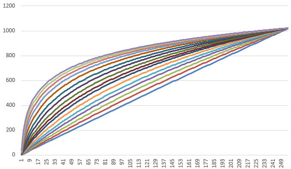
Figure 5-2: Default 16-Line Global Tone Mapping

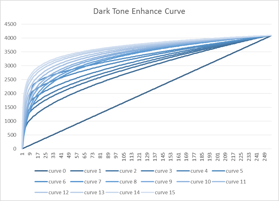
Figure 5-3: Default 16-Line Global Tone Mapping (HDR)

WDRStrByY : Controls WDR strength by Y. Parameter range: 0 ~ 255. The greater the value, the stronger the WDR function.

Strength : WDR global strength. Parameter range: 0 ~ 255. The greater the value, the stronger the WDR function.

Dark / Bright Limit : Limits the WDR function strength. Parameter range: 0 ~ 255. Darkness and brightness are controlled separately. If you do not want the dark pixels to be brightened up too much, a greater DarkLimit value can be set; and if you do not want the bright pixels to be darkened too much, a greater BrightLimit would be suggested.

GammaSyncEn : Enable of WDR sync with Gamma. If disabled, it takes gamma lut in index 0. Connecting Gamma with WDR will get a better WDR effect but if any Gamma curve is set to vary by ISO, flicker might be observed when the Gamma curve is changed. In this case, you may have to disable this function.

5.1.3. Adjustment Steps¶

Enable WDR first, to see whether the default effect is enough.
If the strength is too strong or too weak, adjust the Strength parameter directly.
If brightening over dark pixels is of primal concern, you can further adjust DarkToneEnhance.
If deemed necessary, adjust WDRStrByY or Dark Limit / Bright Limit further.

5.2. WDRCurve¶

This feature, which replaces the Dark Tone Enhance Curve in WDR, allows you to modify the curve by yourself. If the WDRCurve API is enabled, the 16 sets of Curves built in the Dark Tone Enhance in the original WDR API will be controlled by WDRCurve.

It is not recommanded to change the setting by ISO since flicker might occur when the curve is changed. As an alternative, you can tune WDRStrByY and Strength by ISO with a fixed GlobalDarkToneEnhance curve to attain the desired effect.

5.2.1. Adjustment Interface¶

Select WDR from the menu on the left-hand side. You will find the WDRCurve interface to the right of your screen.

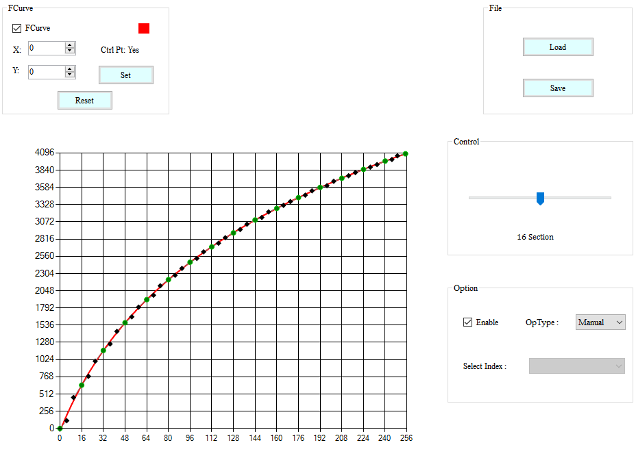
Figure 5-4: WDRCuve Adjustment Interface

5.2.2. Parameter Description¶

Control project is implemented to adjust the number of nodes used to generate the curve.

5.2.3. Adjustment Steps¶

Adjust the curve to achieve proper distribution of bright area and dark area.

5.3. Defog¶

Defog function enables the image to achieve better contrast.

5.3.1. Adjustment Interface¶

Select WDR from the menu on the left-hand side, and the Defog interface will pop up on the screen.

Figure 5-5: Defog Adjustment Interface

5.3.2. Parameter Description¶

Strength : Manually set up the adjustable strength value for contrast, brightness and grayness. Default value is 50.

5.3.3. Adjustment Steps¶

Adjust strength value to achieve a better contrast.

6. DUMMY¶

Dummy API is a default interface, through which new functions will be added, as a way to prevent interfaces from accumulating everytime new functions are added and to avoid such issue affecting the original interface structure. All default values are “-1,” meaning that this certain function is bypassed. If Dummy API is applied and bin files have to be saved, be sure to check “InFile” so that parameters can be properly saved.

6.1. Dummy¶

Supported by ISO adjustment.

6.1.1. Adjustment Interface¶

Select “Dummy” from the menu on the left-hand side, and Dummy interface will appear on the screen.

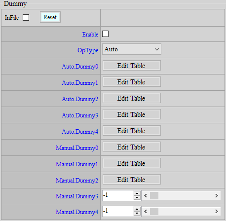
Figure 6-1: Dummy Adjustment Interface

6.1.2. Parameter Description¶

Dummy0 : Currently not functional. Default value is “-1.” Parameter range: -1 ~ 255.

Dummy1 : Strength of NRLuma bilateral filter, with Dummy1[0] representing the level of intensity. Parameter range: 0 ~ 7. Dummy1[1~32] is the weight table, and the horizontal axis represents difference from the center. The smaller the difference is, the greater the weight. Parameter range: 0 ~ 31.

Dummy2 : For the adjustment of SharpnessUD according to the extent of motion. This function is basically the same with “DetailMotOffset” for sharpness. Whereas only one value is subject to adjustment in DetailMotOffset for sharpness and other data will be automatically processed, various adjustments can be made with Dummy2 in accordance with different levels of motion. When Dummy 2 is on, DetailMotOffset for sharpness automatically becomes ineffective, and only Dummy2[0~15] would be functional. Parameter range: 0 ~ 255.

Dummy3 : Currently not functional. Default value is “-1.” Parameter range: -1 ~ 255.

Dummy4 : Currently not functional. Default value is “-1.” Parameter range: -1 ~ 255.

6.1.3. Adjustment Steps¶

Currently not available.

6.2. Dummy_EX¶

Do not support adjustment by ISO.

6.2.1. Adjustment Interface¶

Select “Dummy” from the menu on the left-hand side, and Dummy_EX interface will appear on the screen.

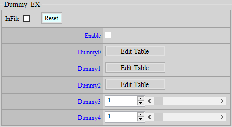
Figure 6-2: Dummy_EX Adjustment Interface

6.2.2. Parameter Description¶

Dummy0 : The nodes of EdgeKillLut on the horizontal axis of sharpness, accumulated by the power of two. Only when the value is set from 0 to 5 will this parameter become functional. Parameter range: 0 ~ 15.

Dummy1 : Enables the results from the NR3D process to come closer to the results from the current frame. Dummy1[0] being the switch. Parameter range: 0 ~ 1. Dummy1[1] is the maximum value of motion. The smaller the value is, the greater the limitation imposed upon the NR3D results to come closer to the current frame. Parameter range: 0 ~ 255. Dummy1[2] is the moving threshold value. In cases where the difference between NR3D result and that of the current frame is smaller than this threshold value, this parameter will not be functional. Parameter range: 0 ~ 255.

Dummy2 : Currently not functional. Default value is “-1.” Parameter range: -1 ~ 255.

Dummy3 : The modes of motion information transmission by NR3D. “0” means direct reference to the difference between current frame and reference frame, while “1” means one extra limitation. When situation changes from dynamic to static, the maximum change of motion information in each frame is 1, showing a slower change in motion. Parameter range: 0 ~ 1.

Dummy4 : Currently not functional. Default value is “-1.” Parameter range: -1 ~ 255.

6.2.3. Adjustment Steps¶

Currently not available.

7. TEMPERATURE SETTING¶

When chip temperature changes, corresponding adjustment can be made to IQ to achieve better visual effects.

7.1. Temperature¶

Set up temperature nodes and corresponding IQ settings.

7.1.1. Adjustment Interface¶

Select Temperature from the menu on the left-hand side, and the Temperature interface will pop up on the screen.

Figure 7-1: Temperature Adjustment Interface

7.1.2. Parameter Description¶

TemperatureLut : Temperature nodes. Up to 16 nodes are supported.

ObcOffset : Offset value of OBC. The larger the value is, the greater the subtraction. Default value is 0.

DynamicDPRatio : Strength change ratio of DynamicDP. The larger the value is, the greater the strength. Default value is 50.

CrosstalkRatio : Strength change ratio of Crosstalk. The larger the value is, the greater the strength. Default value is 50.

NRDeSpikeRatio : Strength change ratio of NRDeSpike. The larger the value is, the greater the strength. Default value is 50.

NR3DRatio : Strength change ratio of NR3D corresponding to MD.Thd and MD.Gain in order. The larger the value is, the greater the strength. Default value is 50.

NRLumaRatio : Strength change ratio of NRLuma. The larger the value is, the greater the strength. Default value is 50.

SharpnessRatio : Strength change ratio of Sharpness corresponding to OverShootGain and UnderShootGain in order. The larger the value is, the greater the strength. Default value is 50.

SaturationRatio : Strength change ratio of Saturation. The larger the value is, the greater the saturation. Default value is 50.

ColorToneRatio : Strength change ratio of ColorTone corresponding to R/G/B in order. The larger the value is, the greater the saturation. Default value is 50.

7.2. Temperature Info¶

Obtain current chip temperature.

7.2.1. Adjustment Interface¶

Select Temperature from the menu on the left-hand side, and the TemperatureInfo interface will pop up on the screen.

Figure 7-2: TemperatureInfo Adjustment Interface

7.2.2. Parameter Description¶

Temperature : Obtain current chip temperature, read only.

8. DAY NIGHT MODE DETECTION¶

Detection of the environmental brightness usually relies on the application of ALS (Ambient Light Sensor), which generates information for users to select from Day mode or Night mode accordingly. This function aims to facilitate the determination of Day/Night mode without using the ALS. By setting customized determining conditions, you can switch between Day mode and Night mode according to the API results.

8.1. DayNightDetection¶

The Day/Night detection API allows user to set respective conditions for the determination of switching from Day mode to Night mode or vice versa, and the detection result will be shown in the DayNightInfo API, which is set out in the next section.

8.1.1. Adjustment Interface¶

Select “Day/Night Mode” from the menu on the left-hand side to find the DayNightDetection interface.

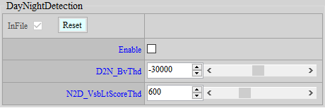
Figure 8-1: DayNightDetection Adjustment Interface

8.1.2. Parameter Description¶

Enable : Switch of the detection function. Information in the DayNightInfo interface will only become effective when Enable is checked.

D2N_BvThd : The threshold value of brightness for determining whether you should switch from Day mode to Night mode. If the current brightness value (accessible as “BV” in AEInfo) falls below this threshold, the D2N flag in the DayNightInfo interface will show “1” and become true. Value range: -1048576 ~ 1048576.

N2D_VsbLtScoreThd : The “Score” threshold for determining the switch from Night mode to Day mode. The Score is calculated by the ratio of visible light to IR light, and a higher value suggests the dominance of visible light in this environment. If the current score (accessible as “N2D_VsbLtScore” in DayNightInfo interface) grows larger than this threshold, the N2D field in the DayNightInfo interface will show “1” and become true. Value range: 0 ~ 2000.

8.2. DayNightInfo¶

This API shows detection result. Please note that this API shows the result only and you should still take actions accordingly, such as loading Day/Night API bin file or controlling IR LED, when necessary.

8.2.1. Interface¶

Select Day/Night Mode from the menu on the left-hand side to find the DayNightInfo interface.

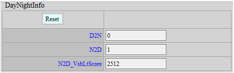
Figure 8-2: DayNightInfo Interface

8.2.2. Parameter Description¶

D2N : Field for determining whether switching to Night mode is necessary. The value “1” means that the current environmental brightness has met the switching condition. Note: The field is only meaningful when the current mode is Day mode.

N2D : Field for determining whether switching to Day mode is necessary. The value “1” means that the current environmental brightness has met the switching condition. Note: The field is only meaningful when the current mode is Night mode.

N2D_VsbLtScore : The score is calculated by the ratio of visible light to IR light, and higher score means visible light is more dominant in the environment. In cases where switching to Day mode is considered desirable, users can read this score to set “N2D_VsbLtScoreThd” in the DayNightDetection Adjustment Interface.

9. NIGHT MODE SETTING¶

When ambient brightness is low to a certain degree, IR light usually will be turned on, and the IR-Cut filter of the lens will be enabled to increase the amount of incoming light. This is in fact a special case, for which certain AE, AWB and IQ settings should be modified accordingly. Due to the use of IR light, Night mode can even apply a very low gain. As such, it is not advised to have Day mode and Night mode share the same bin file and differentiate the two simply by ISO index value. Instead, we suggest that separate bin files be maintained for Day mode and Night mode, respectively. When mode change is determined necessary by the system, you can then load the corresponding bin file. In the following section, we will provide a detailed description of the settings suggested for noise level reduction in Night mode.

9.1. ColorToGray¶

Enabling IR-Cut filter will cause color to get abnormal, so it is a usual practice to turn the screen from color to gray scale.

9.1.1. Adjustment Interface¶

Select ColorToGray from the menu on the left-hand side to find the ColorToGray interface.

Figure 9-1: ColorToGray Adjustment Interface

9.1.2. Parameter Description¶

Enable: Switch to enable color to gray function.

10. RGBIR SENSOR TUNING¶

RGBIR senor is a special type of sensor which, as compared to normal RGB Bayer sensor, features an additional IR pixel for sensing infrared light and uses Dual Band filter instead of IR Cut for IR removal at the backend by way of software method. Our goal in this chapter, therefore, is to provide tips on how to set the IR removal ratio to have the picture exhibit the same color as achieved by the use of IR Cut.

10.1. RGBIR Ratio Adjustment¶

10.1.1. Adjustment Interface¶

Select RGBIR from the menu on the left-hand side to find the RGBIR interface.

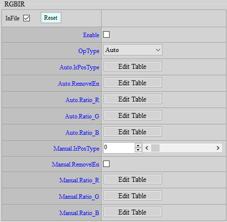
Figure 10-1: RGBIR Adjustment Interface

10.1.2. Parameter Description¶

IrPosType: Used to change the order of sequence of R, G, B, and IR pixels on the sensor. Parameter range: 0 ~ 7.

RemovelEn: IR removal function enable.

Ratio_R: Ratio of R channel IR removal (from dark to bright). Parameter range: 0 ~ 4095.

Ratio_G: Ratio of G channel IR removal (from dark to bright). Parameter range: 0 ~ 4095.

Ratio_B: Ratio of B channel IR removal (from dark to bright). Parameter range: 0 ~ 4095.

10.1.3. Adjustment Steps¶

The RGBIR ratio is associated with OB. So, before adjustment, calibrate OB first.
Set the last value of Ratio_R, Ratio_G, and Ratio_B as 64, and fill out all the remaining blanks with 4095. Observe the image now. If there’s any color deviation, move on to the next step. (It is suggested that you take a picture of the 24-color Color Checker to see whether any color shift occurs at the lower gray scale region and whether the color at the upper region is accurate.)
Keep the last value of the Ratio table as 64 throughout the process of the adjustment, so as to prevent the unexpected decline of brightness in the overexposure region or the unexpected appearance of abnormal color control parameters not within the range of adjustment for normal sensitive region.
Keep Ratio_R and Ratio_B unchanged and adjust Ratio_G to 2000 (all cells in the table from left to right set to 2000, with the exception of the last cell which should retain the value of 64). In this case, the image will appear greenish.
Adjust up Ratio_G gradually, until the gray scale region of the image no longer appears greenish.
Set Ratio_B to 2000. The image will appear bluish now. Then, as in the case of Ratio_G, adjust up Ratio_B gradually, until the gray scale region of the image no longer appears bluish.
Similar to Ratio_G and Ratio_B, lower Ratio_R first and then adjust it up gradually, to make color and gray scale as accurate as possible.
If any particular color or any brightness is suspected to have a problem of color deviation, adjust the associated brightness ratio, noting that the table from left to right corresponds to brightness from dark to bright.

11. AE INTRODUCTION¶

AE is used to control the global image brightness in a desirable state based on the statistical data collected.

11.1. AE Adjustment¶

11.1.1. Adjustment Interface¶

Select AE from the menu on the left-hand side to find the AE Adjustment interface.

11.1.2. Parameter Description¶

< AEState >

AE State: AE state control. Normal AE will put AE in normal operation, and Pause AE will suspend AE operation in the state where it stands at the time of pause and resume normal operation when Normal AE is enabled.
< ManualExposure >

FNx10: Aperture (F number) x 10 (ex: F1.8 => 18)

SensorGain: Sensor gain (1024 = 1x)

ISPGain: ISP digital gain (1024 = 1x)

US: Shutter time, in unit of us
< AEConverge >

ConvThdIn: Inner convergence interval. When AE is in the process of convergence, the screen will be converged until the range of target +- inner convergence interval is reached.

ConvThdOut: Outer convergence interval. The threshold to have AE start convergence again from steady state (current brightness beyond the range of target +- outer convergence interval).

ConvSpeedX: X axis of the convergence speed table, which corresponds to the current brightness (Cur Y). The leftmost position represents the darkest brightness, and the rightmost the brightest. The bottom two squares in the center will automatically align to the current AE target position, so it is not necessary to modify these two squares, which take 470 as the default value. The head and tail squares are set to 0 and 2000 respectively by default.

ConvSpeedY: Y axis of the convergence speed table. Cur Y corresponds to the X axis and then finds the convergence speed (ratio, 0 ~ 1024) of the corresponding Y axis. If the value is set too small, AE response will be slow, and even unable to converge. On the other hand, if the value is set too large, brightness will change very swiftly, and appears blinking when the video is played.
< AEStabilizer >

This function can prevent AE from being easily triggerd by local change in current frame, thereby making the brightnees of the frame stabler. Enable: Switch of this function.

DiffThd: The threshold of the difference between reference frame statistics and current frame statistics. If the Y difference of this statstics block exceeds this threshold, it means this statistics block has changed. On the other hand, if the Y difference of this statstics block is smaller than this threshold, it means there is no change in this statistics block. Data range: 0 ~ 20 (in 8-bit precision), suggested value: 2. Too big value is not recommended, because this will cause brightness change to be not smooth enough when you increase or decrease the brightness of the light soure smoothly.

Percent: The percentage threshold of the frame. When AE is in converged state, if the percentage the brightness-changed area occupies the whole frame is smaller than this value, AE will keep current setting. Data range: 0 ~ 100; the default value is 50.
< AEPlainTbl >

NumOfExpoTblEntry: Sets the number (row) of AE exposure tables.

ExpoTblEntry: Exposure schedule. Setting of Aperture (FNx10), Shutter (us), Total Gain and Sensor Gain in the sequence from left to right, respectively. Brightest on the top and darkest on the bottom.
< AEWinWeight >

Weighting PAGEle ID: Light weighting table ID. Three types of weighting table are supported by default: Average, Center, and Spot.

WindowWeighting: Light weighting table.
< ExposureStrategy>

The parameters in this category are used in combination with AE target settings, to adjust the sensitivity and strength of anti-overexposure when calculating the floating target.

Strategy: Exposure strategy: Auto / dark order first (low light compensation / bright order first (strong light suppression)

Weighting: Variation of strength for dark order first and bright order first. The bigger the weighting, the more intense the variation of strength.

UpperNum: Number of points for upward floating target.

UpperY: Upward floating range. If set to 0, floating target will be disabled and the target will rely solely on the Target Offset setting.

UpperX: The point where the upward floating range corresponds to the BV.

LowerNum: Number of points for downward floating target.

LowerY: Downward floating range. If set to 0, floating target will be disabled and the target will rely solely on the Target Offset setting.

LowerX: The point where the downward floating range corresponds to the BV.

Note: Floating target means the target is automatically calculated based on image histogram change.

Strength: Strength of anti-overexposure mechanism in case of floating target. The greater the value, the stronger the strength (of darkening).

Sensitivity: Sensitivity of anti-overexposure mechanism in case of floating target. The greater the value, the darker the image.
< ExposureStrategyEx >

New version of exposure strategy API. User can design the strategy to prevent over-exposure or under-exposure. AE will follow this strategy to adjust SceneTarget dynamically.

Enable: Switch of this function. If this API is enabled, the ExposureStrategy will not work.

Mode: Exposure strategy mode, inculding Count Mode and Target Mode. If Count Mode is selected, BT (DT)_ThdY and BT (DT)_Percentx10 will work. Users can decide the permillage of the statistical value above (below) the specified brightness threshold as opposed to the total number of statistical values. If Target Mode is selected, BT (DT)_Percentx10 and BT (DT)_Taergetx10 will work. User can decide the average brightness target of the top (bottom) per-mille statistics.

Priority: Priority setting, including BrightTone (over-exposure prevention) and DarkTone (under-exposure prevention).

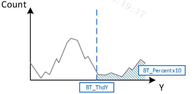
Figure 11-1: AE StrategyEx Count Mode & Bright Priority

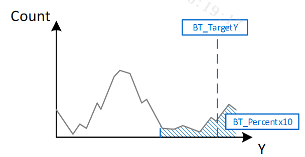
Figure 11-2: AE StrategyEx Target Mode & Bright Priority

BT_NodeNum: The node numbers of Bright Tone.

BT_NodeBV: The BV corresponding to each node of Bright Tone.

BT_ThdY: The brightness threshold of Bright Tone. Data range: 0 ~ 255. It only works on Count Mode.

BT_PercentYx10: The permillage setting of Bright Tone. Data range: 0 ~ 1000. It can work on both strategy modes.

BT_TargetYx10: The average brightness target of Bright Tone. Data range: 0 ~ 2550. It only works on Target Mode.

BT_ MaxOffsetDown: The maximum offset down from AE target. Data range: 0 ~ 2550. Setting it to 0 is equal to disabling over-exposure prevention, and the target will rely solely on the Target Offset setting.

DT_NodeNum: The node numbers of Dark Tone.

DT_NodeBV: The BV corresponding to each node of Dark Tone.

DT_ThdY: The brightness threshold of Dark Tone. Data range: 0 ~ 255. It only works on Count Mode.

DT_PercentYx10: The permillage setting of Dark Tone. Data range: 0 ~ 1000. It can work on both strategy modes.

DT_TargetYx10: The average brightness target of Dark Tone. Data range: 0 ~ 2550. It only works on Target Mode.

DT_ MaxOffsetDown: The maximum offset up from AE target. Data range: 0 ~ 2550. Setting it to 0 is equal to disabling under-exposure prevention, and the target will rely solely on the Target Offset setting.

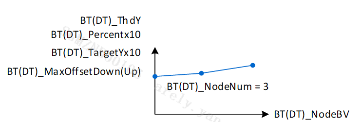
Figure 11-3: All LUTs share the same NodeNum & NodeBV
< AEStrategyExInfo >

GMBlendRatio: The blending ratio for AdaptiveGamma and normal Gamma (Gamma setting on the Gamma page), data range: 0 ~ 1024. This ratio is calculated from final SceneTarget, TargetOffset, max BT_MaxOffsetDown and max DT_MaxOffsetUp. If the ratio is lower than 512, normal Gamma will blend with BTGamma. If the ratio is higher than 512, normal Gamma will blend with DTGamma. If the ratio is 512, normal Gamma will be used. Please refer to the figure below.

Figure 11-4: How GNBlendRatio and AdaptiveGamma Work

UpperLimitTargetYx10: Current upper limit of the floating AE target.

LowerLimitTargetYx10: Current lower limit of the floating AE target.

BTCntPcentx10: Current permillage of total statistics, of which the brightness is higher than BT_ThdY.

DTCntPcentx10: Current permillage of total statistics, of which the brightness is lower than DT_ThdY.

BTYx10: The average brightness of current top BT_Percentx10 per-mille bright statistics.

DTYx10: The average brightness of current bottom DT_Percentx10 per-mille bright statistics.
< AdaptiveGamma >

This function need to work with StrategyEx. It can adjust Gamma dynamically to increase the dynamic range of the image.

Enable: Switch of this function. If this function is disabled, normal Gamma will be used.

BTGamma: If GMBlenRatio is lower than 512, Gamma will blend with BTGamma according to GMBlenRatio.

DTGamma: If GMBlenRatio is higher than 512, Gamma will blend with DTGamma according to GMBlenRatio.
< ExposureMode >

Exposure Mode: AE status control option. Auto for fully automatic exposure, AV_Mode for apperture-first exposure, SV_Mode for gain-first exposure, TV_Mode for shutter-first exposure, and M_Mode for fully manual exposure.
< AETarget >

Target Points Num: Number of points for AE target (AE target varying with different ambient brightness (BV).

Target Offset: AE target at each point.

Target BV: The BV value corresponding to each point.
< EVComp >

EVComp: +- ev brightness compensation function denominator.

Grad: +- ev brightness compensation function numerator.
< ExposureLimit >

MinShutter: Minimum shutter time

MaxShutter: Maximum shutter time

MinFNx10: Minimum aperture value (the greater the value, the smaller the aperture)

MaxFNx10: Maximum aperture value

MinSensorGain: Minimum sensor gain

MinISPGain: Minimum ISP digital gain

MaxSensorgain: Maximum sensor gain

MaxISPGain: Maximum ISP digital gain
< Flicker >

Flicker: Anti-flicker device used for specified frequency. There are four options: Disable, 50Hz, 60Hz, and Auto.
< FlickerEx >

Enable Enables/Disables the anti-flicker function. If FlickerEx is enabled, the old Flicker API will not work.

OpType Anti-flicker work mode: Auto and Manual. When OpType is set to Auto, if flicker is detected, the Flicker type will be changed to the other one automatically. Auto is recommended.

AmpSensitivity Sensitivity of flicker detection (the greater the value, the higher the sensitivity). Parameter range: 0 ~ 100. Suggested setting is 70.

ScoreThd A threshold for auto mode to judge if there is flicker or not. If the Score in FlickerInfo is smaller than this threshold, ValidTimes will add one. If the Score in FlickerInfo is larger than this threshold, the ValidTimes will be reset to 0. Parameter range: 0 ~ 100. Suggested setting is 50.

RefreshCycles Refresh rate for calculating anti-flicker score, this parameter indicates how many cycles are required for updating score once. It usually takes 4 to 7 frames for each cycle. Parameter range: 1 ~ 10. The more cycles, the more reliable score, but the longer time. Suggested setting is 3.

ValidTimesThd In Auto mode, when ValidTimes reaches this threshold, the Flicker mode will be changed to the other one automatically. Parameter range: 1 ~ 10. The more cycles, the more reliable score, but the longer time. Suggested setting is 2.

Flicker Anti-flicker type: 60Hz = 0, 50Hz = 1.
< FlickerInfo >

IsEffective Indicates whether the current flicker detection is effective (1: Effective; 0: Not effective).

FlickerType Anti-flicker type: 60Hz = 0, 50Hz = 1.

Score Obtains the score of current effective flicker detection.

→ If the score is higher, it is judged as the current anti-flicker frequency mode.

→ If the score is lower, it is judged as another anti-flicker frequency mode.
< RGBIR AE >

Enable: Enables/Disables RGBIR AE

MaxYWithIR: Maximum value of bright area average brightness before IR removal.

MinISPGainCompRatio: Maximum ratio of raw image brightness compensation via ISP gain. The smaller the number, the greater the compensation ratio.
< DebugLev >

AE Debug Level: AE debug log output setting. (0: Disable, 1: Exposure, 2: Algo parameters, 4: Algo statistics, 32: API debug, 64: Exposure-2.)
< AE HDR Ratio> - HDR mode only

AE HDR Points Num: Sets the number (row) of AE HDR ratio table

HDR Ratio: Sets the long/short exposure ratio in HDR mode (1024 = 1x)

By Total Gain: Sets the X axis of HDR ratio table, HDR ratio can be different by total gain value (default: 1024, 2048, 4096, 8192...)
< AEPlainShortTbl> - HDR mode only

NumOfExpoTblEntry: Sets the number (row) of AE short exposure table

ExpoTblEntry: Exposure schedule. Setting of Aperture (FNx10), Shutter (us), Total Gain and Sensor Gain in the sequence from left to right, respectively. Brightest on the top and darkest on the bottom.
< ManualShortExposure> - HDR mode only

FNx10: Aperture (F number) x 10 (e.g.: F1.8 => 18)

SensorGain: Sensor gain (1024 = 1x)

ISPGain: ISP digital gain (1024 = 1x)

US: Shutter time, in unit of us

12. AWB INTRODUCTION¶

Since the photographic characteristics of R, G, B pixel are different, the gray scale will have some color shift when viewed under different light sources. The purpose of AWB function is to automatically provide R B gains for compensation, so that the R, G and B values are as similar to one another as possible in the gray scale region.

12.1. AWB Adjustment¶

The AWB statistics are obtained by dividing the screen into 128x90 blocks, each block containing R/G/B value. The default horizontal axis is subsampled to reduce the computation, and hence the statistical values actually computed are 64x90. If you want to check the statistics of a certain scene, open the AWB Analyzer plugin, and click Update to update to the current statistics. The horizontal axis represents (R/G)x100, and the vertical axis (B/G)x100. Therefore, each block can calculate a set of coordinates with its own R, G, and B values, and display the drop point on the chart with a green dot.

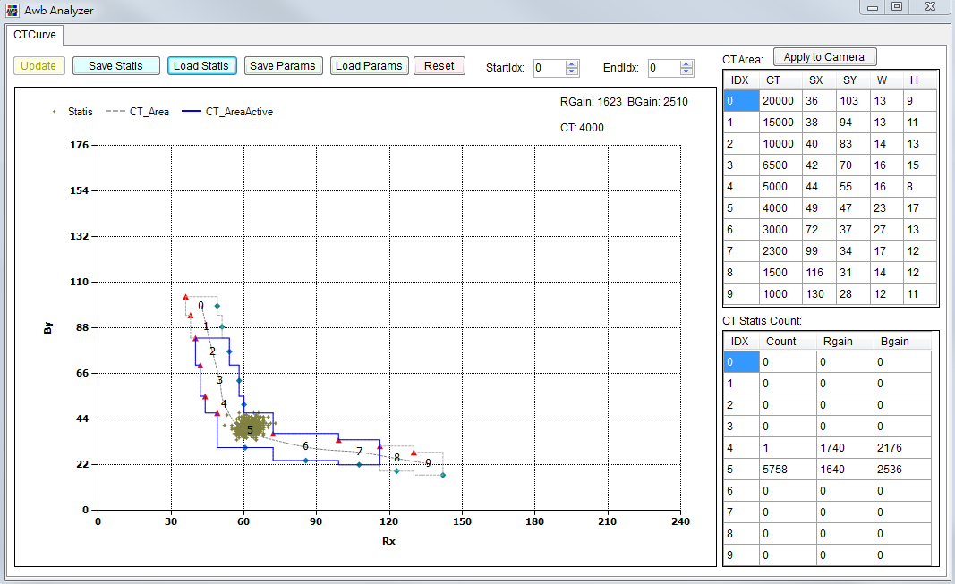
Figure 12-1: Using AWB Analyzer to Analyze Statistic Data

12.1.1. Adjustment Interface¶

Select AWB from the menu on the left-hand side to find the AWB Adjustment interface.

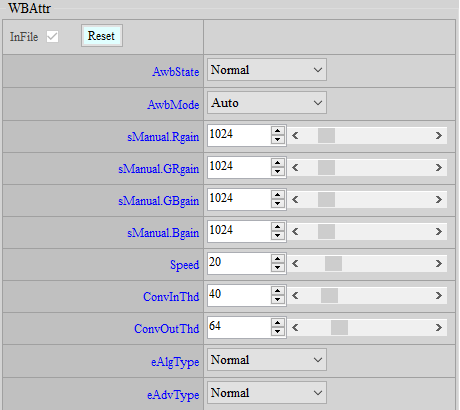
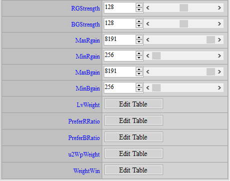
Figure 12-2: Basic AWB Adjustment Interface

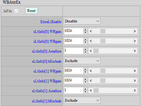
Figure 12-3: AWB Advanced Mode Adjustment Interface

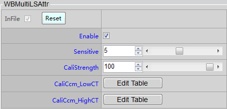
Figure 12-4: AWB Mixed Color and Color Shift Calibration Setting Interface

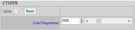
Figure 12-5: CTMWB Setting Interface

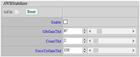
Figure 12-6: AWB Stabilizer Interface

12.1.2. Parameter Description¶

< WBAttr >

Parameters suggested for modification

AwbState : AWB state control option. Normal AWB will put AWB in normal operation, and Pause AWB will suspend AWB operation in the state where it stands at the time of pause and resume normal operation when Normal AWB is enabled.

AwbMode : WB state control option. Auto means AWB, and Manual means MWB.

sManual.R/GR/GB/Bgain : When AwbMode is set to Manual, these four gain values will be applied directly. Parameter range: 0 ~ 8191, 1024 means 1x.

Speed : AWB convergence speed control. Parameter range: 1 ~ 100. The greater the value, the quicker the convergence speed. Default value is 20.

ConvInThd : Convergence interval size control. Parameter range: 0 ~ 255. The greater the value, the easier the convergence. Greater values tend to have a larger gap with the target, while smaller values can cause AWB to be unstable. Default value is 32.

ConvOutThd : The debounce threshold to allow WB recalculation. Parameter range: 0 ~ 255. The value should not be too large, since WB calculation can fail when the light source is changed, thereby causing color deviation. Default value is 64.

eAlgType : AWB algorithm type selection. There are four types to choose from:
1. GrayWorld: Use all AWB statistics to calculate the WB gain.
2. Normal: Use the AWB statistics located at the first two or three CT blocks having the highest count to calculate the WB gain.
3. Balance: Use the AWB satatistics located at all effective CT blocks to calculate the WB gain.
4. Focus: WB gain calculation will focus on single color temperature.
eAdvType : WBAttrEx function enable/disable. WBAttrEx functions only when Advance is chosen. The default is WBAttrEx off.

RG/BG Strength : Global gain for R and B. This parameter will multiply the calculated R/B gain by the specified gain. Parameter range: 0 ~ 255, 128 means 1x.

MaxRgain/MaxBgain : High color temperature R and B gain limit. Parameter range: 0 ~ 8191.

MinRgain/MinBgain : Low color temperature R and B gain limit. Parameter range: 0 ~ 8191.

LvWeight : Color temperature weight setting for different ambient brightness. The greater the weight, the higher the proportion of the color temperature will occupy when calculating R/B gain. Parameter range: 1 ~ 255.

PreferR/Bratio : R/B ratio under various ambient brightness. This ratio will be multiplied in the target R/B gain. Parameter range: 1 ~ 255.

u2WpWeight : The weight to be judged as a reference white pixel. The higher the weight, the easier it is to be chosen as a reference white pixel. Parameter range: 1 ~ 400, the default value is 100.

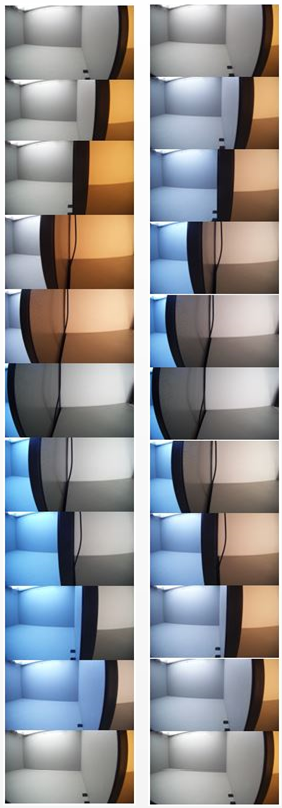
Figure 12-7: Comparison of bWpWeightEnable On/Off Effect (L: On / R: Off)

WeightWin : The image is divided into 9x9 windows and the weight of each window can be given separately. The higher the weight, the grayer the region of window will become. The range is 0 ~ 16. The weight is relative and not absolute in nature; that is, setting 1 or 16 to all windows basically has the same effect. When the lens is fixed and you know exactly which area of the picture should be applied with white balance, this function can be used to make adjustments.
< WBAttrEx >

WBAttrEx series parameters work only when eAlgType is set to Advance. These parameters are mainly used to allow users to define special areas and decide whether to include or exclude statistics falling within those special areas. There are 4 groups of settings available.

ExtraLtEnable : Special color temperature area enable/disable. Must be set to “Enable” to have the special color temperature area come into effect.

sLtInfo.WR/Bgain : R/B gain represented by the center coordinates of special color temperature area. Parameter range: 0 ~ 8191. For conversion, use AWB Analyzer to analyze the drop point of the statistical values, and then move the index to the center of the area to be selected to check the coordinates. Suppose coordinate Rx = 40 and By = 60, divide the coordinate by 100 (0.4, 0.6) and get the reciprocal (1/0.4, 1/0.6). Finally, multiply the coordinate by gain base 1024 (WRgain=2560, WBgain=1706).

sLtInfo.AreaSize : Special area size. Parameter range: 1 ~ 32. 32 means the area extends from center to top, bottom, left and right by 16.

sLtInfo.bExclude : Special area mode selection. Include means statistical values within special area will be counted as reference statistics, and Exclude means statistical values within special area will be ignored.
< WBMultiLSAttr >

This function works only when “Focus” is selected for eAlgType. When eAlgType is “Focus”, the R, B gain of AWB will be based on the reference white pixel, wherever possible. For mixed-light scene in this case, the end farther from the reference white pixel will have apparent color shift. To weaken the color shift, you can enable this function, but then the color phase of the other colors might change. The following diagram illustrates a comparison of the WBMultiLSAttr on/off effect.

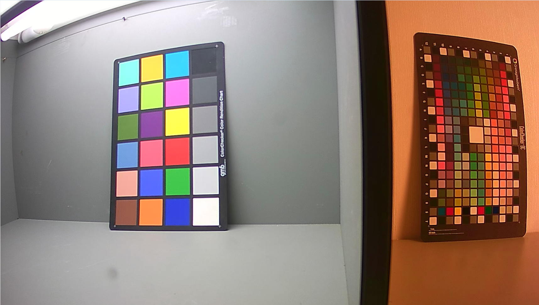
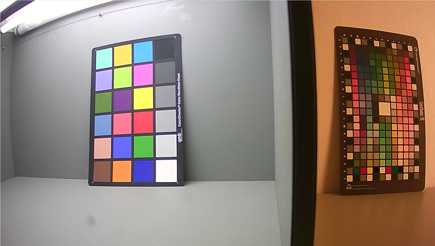
Figure 12-8: Comparison of WBMultiLSAttr Function On/Off Effect (L: Off / R: On)

Enable : Mixed-light color shift calibration function enable/disable. When enabled, the color shift can be mitigated, but the colors within the AWB gray scale area will have some color shift.

Sensitive : Sensitivity of mixed-light judgement. Parameter range: 1 ~ 10. The greater the value, the easier it is to judge the scene as a mixed-light scene.

CaliStrength : Mixed-light color shift compensation strength control. Parameter range: 0 ~ 100. 100 means 1x, i.e. the original CaliCcm strength.

CaliCcm_LowCT : In mixed-light cases, when AWB intends to balance high color temperature, CCM will be used to alleviate the color shift problem occurring at low color temperature area. For now, only the first and third rows are available for adjustment. Nothing will happen if you adjust the second row. The CCM strength is mainly used for mixed lights that come from StartInd and EndInd. The strength actually applied will be based on the ratio of the distance between the two light sources and the distance between StartInd and EndInd.

CaliCcm_HighCT : In mixed-light cases, when AWB intends to balance low color temperature, CCM will be used to alleviate the color shift problem occurring at high color temperature area. For now, only the first and third rows are available for adjustment. Nothing will happen if you adjust the second row. The CCM strength is mainly used for mixed lights that come from StartInd and EndInd. The strength actually applied will be based on the ratio of the distance between the two light sources and the distance between StartInd and EndInd.

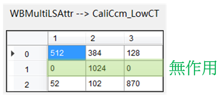
Figure 12-9: CaliCcm_LowCT Interface

Taking CaliCcm_LowCT as an example, our suggestion for CaliCcm adjustment is as follows:
1. Turn on the light box of D65 (or a light source closer to StartIdx, if any), to allow AWB to balance the color temperature.
2. Switch AWB to PAUSE.
3. Change the light box to F (or a light source closer to EndIdx, if any) and adjust CaliCcm_LowCT. While adjusting, be sure to go back to the light source before color temperature balancing from time to time, to see if the normal colors have any excessive color shift. Stop when both have reached a balanced state.
< CTMWB >

CTMWB comes into effect only when Manual is selected for AwbMode of WBAttr. User might apply corresponding WB gain by setting color temperatures.

ColorTemperature : Designated color temperature setting. Parameter range: 1000 ~ 20000.
< AWBStabilizer >

When the environment is stable but AWB is continuously triggered, causing constant flickering of screen color, it is recommended that you enable this function to stabilize AWB changes.

Enable : Enable AWB Stabilizer.

GlbGainThd : The threshold value of global change in WB gain. When AWB is converged, it can only be re-triggered when two conditions are met: the original requirement, which is set out in the description of ConvOutThd parameter; and that the global change in WB gain exceeds this threshold value. Parameter Range: 0 ~ 512. We recommend that you set this threshold to the same value of, or slightly smaller than, ConvOutThd. Default value is 64.

CountThd : The threshold value of continuous count that determines AWB to be re-triggered. If the value is 2, AWB will be re-triggered only if the two conditions are met three times in a row, otherwise AWB will stay stable. Parameter range: 0 ~ 100. Setting the value too large is not recommended because higher value would delay the response time for AWB to be re-triggered.

Default value is 2.

ForceTriGainThd : A threshold value of gain used for mandatorily triggering AWB. This parameter aims to prevent the response time of AWB from being delayed by CountThd in the situation where environmental color temperature or light source drastically changes. If the change of gain meets the re-triggering condition, and the amount of change is greater than this threshold, CountThd will be ignored and AWB will be directly triggered. Parameter range: 0 ~ 8191.

Default value is 150.
< DebugLev >

AWB Debug Level : Set AWBDebug log output.

1: Show simple algo paramaters;

2: Always show detailed algo parameters;

3: Show detailed algo parameters;

7: User Parameters.

12.2. AWBInfo¶

This interface will display the current AWB information. Click ReadPage to update to the latest information.

Figure 12-10: AWBInfo Interface

IsStable : Shows whether AWB is stable or not

WB_Rgain : R gain used by current WB

WB_Grgain : GR gain used by current WB

WB_Gbgain : GB gain used by current WB

WB_Bgain : B gain used by current WB

WB_CT : Environmental color temperature detected at present

The following parameters function only when “Focus” eAlgType is chosen:

WPInd : Current reference white pixel index

MultiLS_Detected : Shows whether mixed-light scene is detected

MultiLS_FirstLSInd : Represents the largest mixed-light source index*2. The actual light source index must be divided by 2. For instance, if index is 8, the actual light source index would be 4, and if index is 9, the actual light source index would be 4.5. The decimal point .5 means the light source falls between color temperature ranges 4 and 5.

MultiLS_SecondLSInd : Represents the second largest mixed-light source index*2. The actual light source index must be divided by 2. For instance, if index is 8, the actual light source index would be 4, and if index is 9, the actual light source index would be 4.5. The decimal point .5 means the light source falls between color temperature ranges 4 and 5.

Figure 12-11: MultiLS_FirstLSInd & MultiLS_SecondLSInd

13. AF INTRODUCTION¶

The purpose of AF is to focus the screen in an ideal state through the received statistical values.

13.1. AF Adjustment¶

13.1.1. Adjustment Interface¶

Select AF from the menu on the left-hand side to find the AF Adjustment interface.

13.1.2. Parameter Description¶

< AF_HWROIMODE>

Mode : ROI mode control option. If the Mode is set to Normal, the screen can be divided into 16 sets of ROI blocks. The window size and position can be set according to user preference. If the Mode is set to Matrix, the screen can be divided into 16 * N sets of ROI windows. The window size and position are relatively more limited.

VerticalBlockNumber : Effective only when the Mode is set to Matrix, this parameter can divide the window into 16 * N sets of ROI blocks (N VerticalBlockNumber).
< AF_HWWIN>

Win : Coordinates of the 16 ROIs, in the sequence x_start, y_start, x_end, y_end.
< AF_HWFILTERATTR>

IIR1 : IIR high filter coefficient.

IIR1_Clip : IIR high filter coefficient input/output limit.

IIR2 : IIR low filter coefficient.

IIR2_Clip : IIR low filter coefficient input/output limit.

IIR1_E1_En : IIR high 2-tap serial filter switch.

IIR1_E1 : IIR high 2-tap serial filter coefficient.

IIR1_E2_En : IIR high 4-tap serial filter switch.

IIR1_E2 : IIR high 4-tap serial filter coefficient.

IIR2_E1_En : IIR low 2-tap serial filter switch.

IIR2_E1 : IIR low 2-tap serial filter coefficient.

IIR2_E2_En : IIR low 4-tap serial filter switch.

IIR2_E2 : IIR low 4-tap serial filter coefficient.
< AF_HWFILTERSQ>

SobelYSatEn : Sobel filter Y threshold switch.

SobelYThd : Sobel filter Y threshold. It takes effect only when SobelYSatEn is true. Pixels with brightness lower than this threshold will be included in the Sobel filter calculation.

IIRSquareAccEn : IIR filter enhanced control switch.

SobelSquareAccEn : Sobel filter enhanced control switch.

IIR1Thd : IIR high filter threshold. The output value will be subtracted by this value before output.

IIR2Thd : IIR low filter threshold. The output value will be subtracted by this value before output.

SobelHThd : Sobel H filter threshold. The output value will be subtracted by this value before output.

SobelVThd : Sobel V filter threshold. The output value will be subtracted by this value before output.

AFTblX : IIR/Sobel filter nonlinear mapping horizontal axis node, which is accumulated to the power of two.

AFTblY : IIR/Sobel filter nonlinear mapping vertical axis node.
< AF_ATTR>

State : State control option. If set to Normal, AF will be under normal operation. If set to Pause, AF will remain in the state when Pause is set, and resume normal operation when switched back to Normal.

Mode : Mode control option. If set to Manual, this parameter will set the motor position directly. If set to Auto, this parameter will conduct auto focus based on the algorithm chosen.

ManualMotorPos : Effective only when Mode is set to Manual, this parameter can directly set the motor position.

Algo : Effective only when Mode is set to Auto, this parameter currently supports the following two algorithms:
OneShot: Scan all spots in one shot and stay at the spot with maximum statistical value.
Continuous: Detect environmental changes dynamically and refocus if any change is detected.
< AF_MOTOR>

MinMotorPos : Minimum Motor position.

MaxMotorPos : Maximum Motor position.

MinMotorStep : The minimum step that the Motor can move within one frame.

MaxMotorStep : The maximum step that the Motor can move within one frame.
< AF_ACC_WEIGHT>

WinNumX : X-direction window number.

WinNumY : Y-direction window number.

EqualWinWgtEn : Statistics value equal weight switch.

WinWgt : Statistical value weight table, which takes effect only when EqualWinWgtEn is false.

IIRHBlendEn : IIRH blending switch. The blending will be performed on the basis of the following three variables.

IIRHWgt_FirstBlendIIRL : IIRH will be blended with IIRL first, as the IIRH ratio.

IIRHWgt_SecondBlendSBLV : IIRH will then be blended with SobelV, as the IIRH ratio.

IIRHWgt_ThirdBlendSBLH : IIRH will finally be blended with SobelH, as the IIRH ratio.
< AF_ONESHOT> , effective only when Algo is set to OneShot

AccSel : Stats type.

MotorStep : Motor step for each frame.
< AF_SCENE_CHANGE>, effective only when Algo is set to Continuous

PreAccSel : Type of statistical value. Determine whether the environment has changed according to the difference of statistical value from the previous frame.

PreAeAccDiffThOft : Luma difference ratio threshold. Will count the total number exceeding this threshold.

PreAeAccDiffThSlp : Luma difference ratio threshold slope. The threshold can be increased by motor step.

PreAeAccCntThOft : Luma total ratio threshold. The environment will be judged as unstable if greater than this threshold.

PreAeAccCntThSlp : Luma total ratio threshold slope. The threshold can be increased by motor step.

PreAfAccDiffThOft : PreAccSel difference ratio threshold. Will count the total number exceeding this threshold.

PreAfAccDiffThSlp : PreAccSel difference ratio threshold slope. The threshold can be increased by motor step.

PreAfAccCntThOft : PreAccSel total ratio threshold. The environment will be judged as unstable if greater than this threshold.

PreAfAccCntThSlp : PreAccSel total ratio threshold slope. The threshold can be increased by motor step.

FocusAccSel : Type of statistical value. Determine whether the environment has changed according to the difference from the previous end-of-convergence value.

FocusAeAccDiffTh : Luma difference ratio threshold. Will count the total number exceeding this threshold.

FocusAeAccCntTh : Luma total ratio threshold. The environment will be judged as unstable if greater than this threshold.

FocusAfAccDiffTh : FocusAccSel difference ratio threshold. Will count the total number exceeding this threshold.

FocusAfAccCntTh : FocusAccSel total ratio threshold. The environment will be judged as unstable if greater than this threshold.

StableCntTh : Continuous stable frame count threshold. The environment will be judged as stable and the motor will be moved to perform auto focus if greater than this threshold.
< AF_SEARCH_START > , effective only when Algo is set to Continuous

SearchMotorStep : Motor step for each frame.

SearchMotorDirByPosTh : Decide the direction of movement according to the current motor position. If greater than this value, will move toward smaller position, and vice versa.

SearchAccSel : Type of statistical value.
< AF_SEARCH >, effective only when Algo is set to Continuous

MinMaxAccRatioPeakThOft : Min-Max value difference ratio threshold, used to determine the peak.

MinMaxAccRatioPeakThSlp : Min-Max value difference ratio threshold slope. The thresold can be decreased according to the total path travelled.

AccDecCntPeakTh : Threshold for the number of consecutive declines in statistical values, used to determine the peak.

NowFakeMaxAccRatioPeakTh : Statistic value decrease proportional threshold, used to determine the peak.

AccDecCntWrongDirTh : Threshold for the number of consecutive declines in statistical values, used to determine if the direction is wrong.

NowFakeMaxAccRatioWrongDirTh : Threshold for the decline ratio of statistical values, used to determine if the direction is wrong.

Note 1: The condition for judging a peak is
if ( (MinMaxAccRatioPeakThOft, MinMaxAccRatioPeakThSlp) &&

(AccDecCntPeakTh || NowFakeMaxAccRatioPeakTh) )

Note 2: The condition for judging a wrong direction is
if (AccDecCntWrongDirTh || NowFakeMaxAccRatioWrongDirTh)

14. IQTOOL INTERFACE CONNECTION FUNCTION OPERATION¶

14.1. IQTool Interface Connection Function Operation Steps¶

Set up the EVB network function, by entering the following command at the terminal:
```
#ifconfig eth0 hw ether 00:xx:xx:00:00:01

#ifconfig eth0 up

#udhcpc

#mixer -n 1 -q
```
Wherein, -q means turning on iqserver, which allows IQTool to be connected.
Select product type:
1. IP Camera
2. Car Camera
Input the IP address of the EVB.
Click the Connection icon

()

to establish the connection. If the icon is changed to (

), which means connection done successfully, then you can start using the tool to adjust image parameters. If you click the icon (

) once again, it will change back to (

), and the connection will be disconnected. An illustration of the setup steps is shown in Figure below.

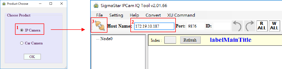
Figure 14-1: IQTool Interface Connection Setup

15. IQTOOL INTERFACE FUNCTION DESCRIPTION¶

15.1. IQTool Interface¶

As displayed in the following Figure, the functions encircled in red dotted line to the left of the IQTool interface are functional tree structures, each node being itself an API collection. Clicking on a node will generate the interface as shown on the right. If you click on the node AE, for example, the associated API — ManualExposure, in this case — will be unfolded dynamically on the right. You can then adjust the API settings in real-time in this interface.

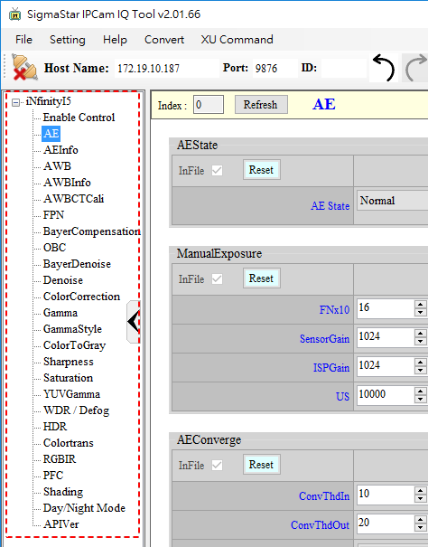
Figure 15-1: IQTool Functional Tree Diagram

15.2. Parameter Tuning¶

Different APIs have different types of parameter setting methods, for example filling-in of values, drop-down menu, reading of values, form creation, etc.

Depending on the initial setting of the APIs, some grant both Read and Write access permissions, others Read only.

Parameter tuning types:

Value: The value can be modified by the following three methods:
- Click on the up/down arrows to adjust the value
- Fill in the value in the associated field
- Move the scroll bar leftward/rightward to adjust the value
Value-type parameter tuning will have a prescribed range for adjustment, with min/max value set according to the API’s initial setting. Take ManualExposure as an example, the min. value of FNx10 is 10 and the max. 220. If the value filled in is smaller than 10, the tool will auto-correct it to 10; if the value filled in is greater than 220, the tool will auto-correct it to 220.

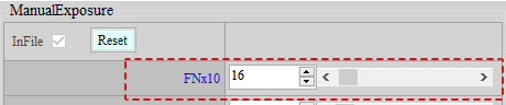
Figure 15-2: Value
Drop-Down Menu: By clicking on the down arrow, you will see the drop-down menu with options for you to choose from. For example, in the API AE ~ Flicker shown in Figure below, you can select Disable, 60Hz, or 50Hz as the value for the Enable field.

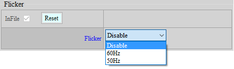
Figure 15-3: Drop Down Menu
Reading of Values: The value shown in this type of parameter setting is read-only and non-writable. Take API AWBInfo in Figure below as an example, the value of 2130 shown in the WB_Rgain field can be read but not written.

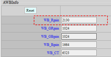
Figure 15-4: Reading of Value
Form: A button is provided on the API, for example the Edit Table button shown in Figure below.

Figure 15-5: Button for Popping up a Table for Editing

By clicking on the button, you will see a form window (Pop-up Form Window in Figure below), with a Table inside the window. Click on the Read button to read the value from the platform, and the Write button to write the value to the platform.

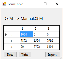
Figure 15-6: Pop-up Form Window

If the table is read-only, write to the platform will not be permitted by API, then only the Read button will be shown.

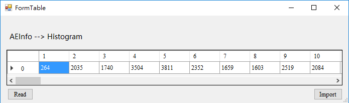
Figure 15-7: Read-only Form Window

15.3. Data Read/Write¶

You can read/write data of the entire API collections, or data of all APIs under the current page. Let’s take the case shown in Figure below, where the current page is API AE, as an example. If you press the Read Page on the upper right corner, all data under the current AE page will be read out; if you press the Write Page on the upper right corner, all data will be written into the current AE page. On the contrary, if you press the R ALL button, all data of the entire API collections, not just those of the API AE, will be read out; if you press the W ALL button, all data will be automatically written into the entire API collections, except those concerned with Gamma/Calibration. For Gamma, you must manually select the Write Page to enable data to be written to the API. Table 1 shows details on the icons used for data read/write.

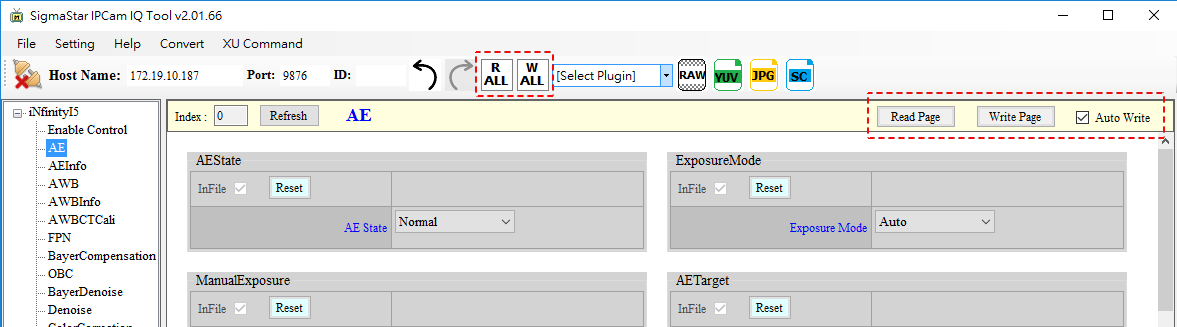
Figure 15-8: Data Read/Write

Table 1: Description of the Data Read/Write Icons

Icon	Function	Description
	Read data of all API collections	Pressing this button will read data of all API collections
	Write data to all API collections	Pressing this button will write data to all API collections (except Calibration)
	Read data of current page	Pressing this button will read all API data under the current page
	Write data of current page	Pressing this button will write all data to API under the current page
	Write data of current page to API in real-time	When checked, will enable the Auto Write function

15.4. Saving Images in Raw/YUV/JPG Format¶

Once the platform is connected, you can use the buttons encircled in red dotted line to capture images in four formats.

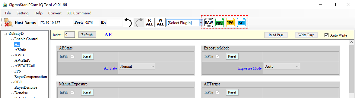
Figure 15-9: Saving Images

When the capture starts, a new window will be opened to display the progress. If the image is captured successfully, a success message will be shown, together with the directory where the image is saved. The default path is the ./Image folder under the directory where the program exists.

Figure 15-10: Image Saved Successfully

15.5. Creating, Loading, Saving Parameters¶

During tuning of the IQTool, you can save the parameters of the current page to specified directory or load any parameter files already saved at any time.

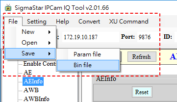
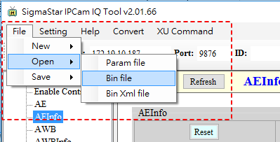
Figure 15-11: Creating, Loading, Saving Parameters

IQTool has the function of automatically saving Bin file. The unit of the parameter is minutes. 0 means no automatic storage. The Bin File will be stored in the CvtXml folder, as shown in Figure 15-12. With manual saving, the seconds will be repeated, as shown in Figure 15-13.

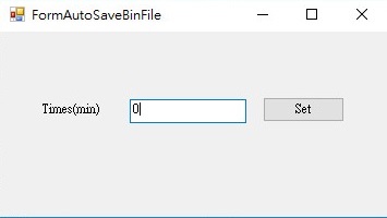
Figure 15-12: Schematic Diagram of Automatically Saving Bin File

Figure 15-13: Showing the Remaining Time until Auto-Saving the Next Bin File

When saving an API Bin file, it is possible to save the file without API by unchecking the corresponding InFile box.

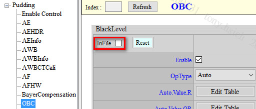
Figure 15-14: InFile Function

Two formats are available for saving parameter files: Xml and Bin.
- Xml:
  
  Xml is mainly used to save GUI (including interface parameters) of the tool.
- Bin:
  
  Bin is for saving API parameters only. You can call MI_ISP_API_CmdLoadBinFile(MI_U32 Channel, char* filepath, MI_U32 user_key) at application layer to automatically load the API parameters.
- Magic Key: can be used to verify if the bin file matches with the device. The Magic Key can be set up via the Setting page.
  
  Subsequent to the API parameters of the bin file, the Xml file of the corresponding serial port will be added to ensure Xml file is matched with the API parameters.
Three formats are available for loading parameters: Xml, Bin and Bin Xml.
Xml:

Xml is used to load GUI (including interface parameters) of the tool.
Bin:

Bin is for loading API parameters.
Bin Xml:

Bin Xml is used to load API parameters and to add Xml of the corresponding serial port.

15.6. Gamma Tuning¶

Click on the Gamma tree node, and the associated Gamma tuning interface will be shown on the right.

Figure 15-15: Gamma Tuning Interface
For a quick overview of the Gamma interface functions, please refer to Figure 15-16.

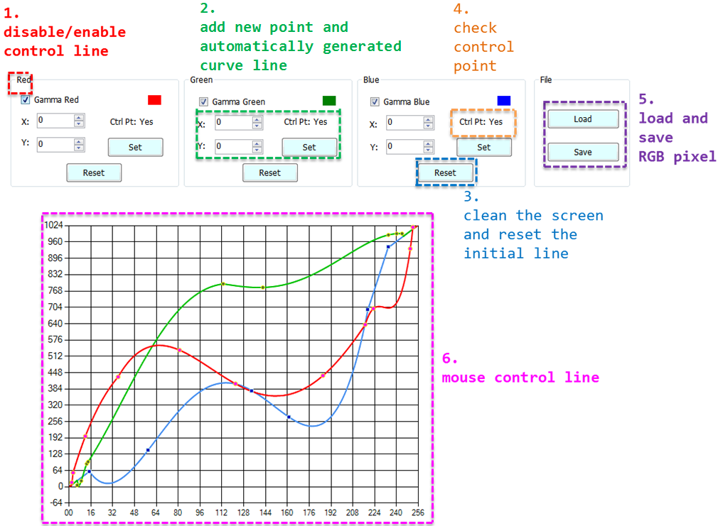
Figure 15-16: Gamma Interface Function Overview

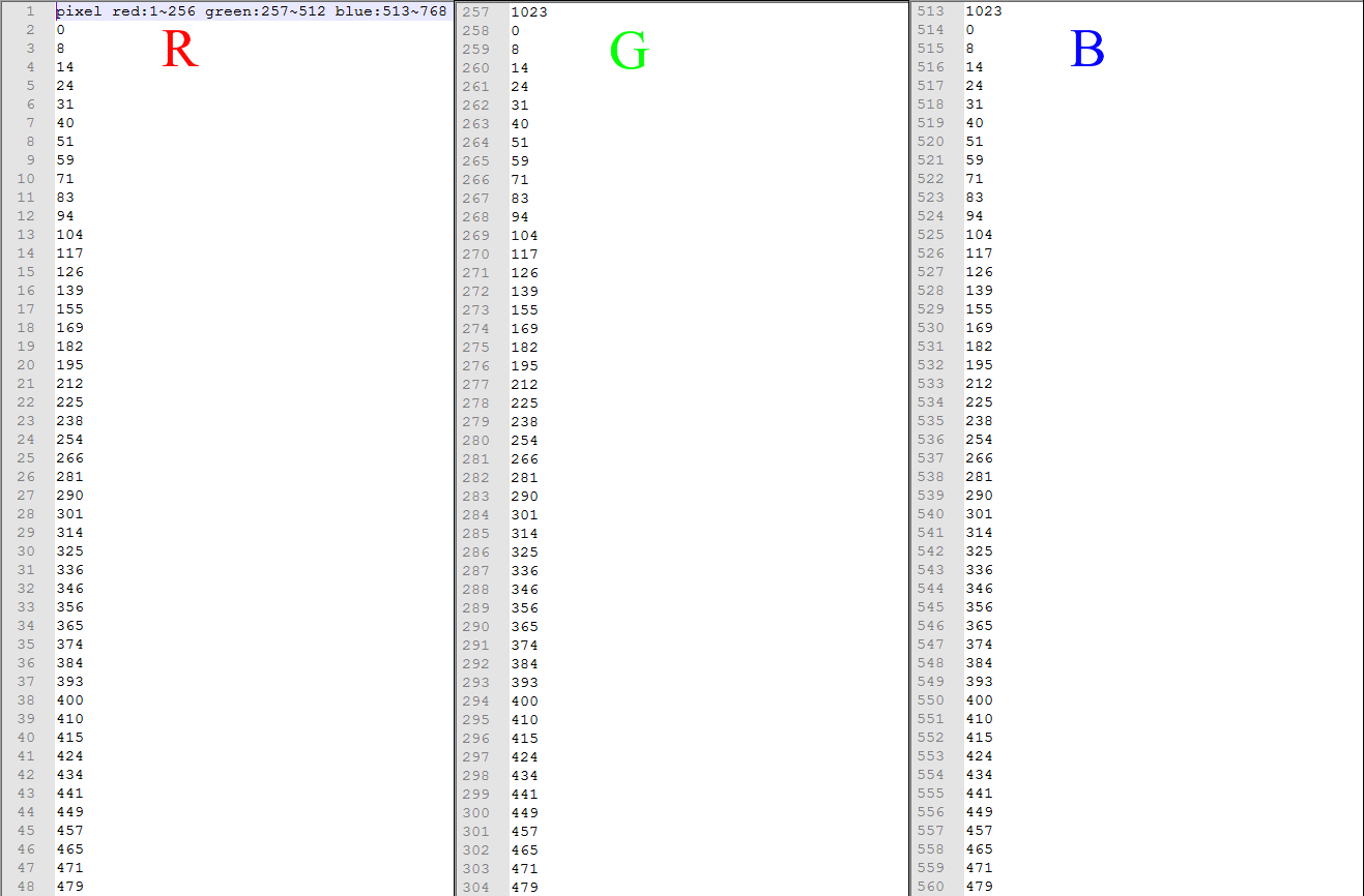
Figure 15-17: Gamma File Saving and Reading Format
For a detailed description of the Gamma functions, please refer to Table 2.

Table 2: Detailed Gamma Function Descriptions

	Function	Description
1	Disables/Enables R,G,B control line	If Gamma Red is checked, the red line will be mouse-controllable and tangible. - If Gamma Red is not checked, the red line will be mouse-uncontrollable and intangible. - The same applies to Gamma Green and Gamma Blue.
2	Adds new point and automatically generates curve line	Move the up/down arrow to adjust the X axis and Y axis values (or input the desired values in the fields), then press the Set button: - If there is no control point yet, new (x,y) control points will be added on the curve line and a smooth curve will be formed based on the newly added control points. - If a control point already exists on X axis of the curve line, the control point will take the Y axis value inputted and a smooth curve will be formed.
3	Resets the initial line	Clear the R, G or B line, and restore the initial setting (bypass gamma).
4	Checks the control point	“Yes” if a control point has been successfully created, “No” otherwise.
5	Loads and saves RGB pixel	Load: Load the txt file bearing RGB pixel values, and an RGB curve line will be generated automatically. - Save: Save the RGB curve line pixel values as a txt file. See Figure 15-17. - The file format is: R->G->B header: 0 (description) pixel red: 1 ~ 256 pixel green: 257 ~ 512 pixel blue: 513 ~ 768
6	Mouse control page	Left click on the curve line to add a new control point. Move the control point and the auxiliary point to create a smooth curve line. - Right click on the control point to delete it.
7	Control point option	If Sync RGB is checked, the R, G and B curve lines will merge into one gray line. Modifying this gray line will modify the R, G and B lines at the same time. - Drag the Section Bar leftward/rightward to set the number of control points for the curve line.

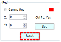
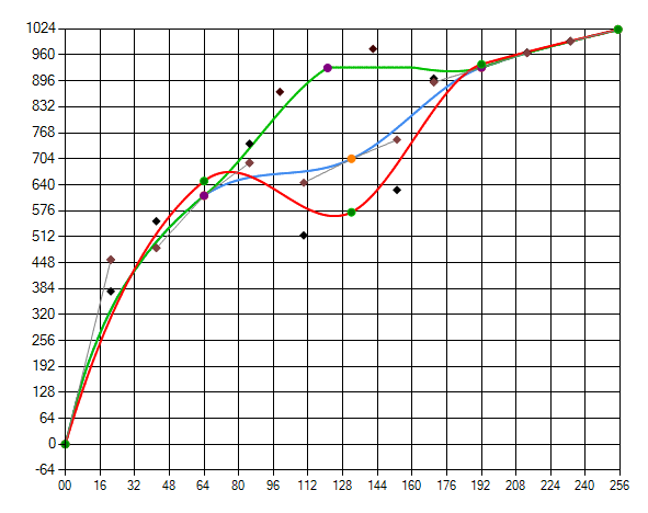
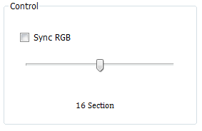
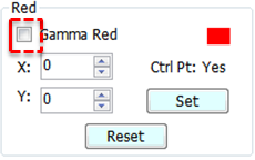
Method to adjust Gamma curve line: The R, G and B curve lines will be shown on the coordinates when initialized. With Gamma Red, Gamma Green and Gamma Blue checked, you can use your mouse to control movement of the cross symbol and click on the control line. If the spot you click on happens to be where the three curve lines overlap, the priority will be Red, Green and then Blue. Let’s take R curve line as an example. You can left click on the mouse to add a new control point and right click to delete it. Moving the control point can modify the curve line. Two auxiliary points are provided beside the control point, to help fine tune the Bezier curve. There are 256 pixel values each for R, G and B.

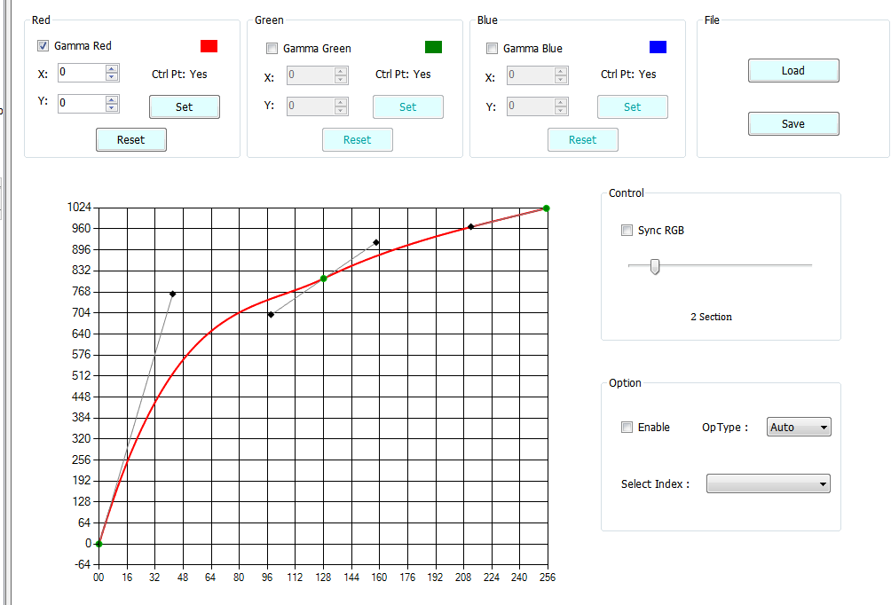
Figure 15-18: Gamma Curve Line Adjustment
Gamma Curve Line Read Page and Write Page:
- Read Page: The get API. Pressing the Read Page button will get the value on the curve and send it to the platform.
- Write Page: The set API. Pressing the Write Page button will write the value on the platform to the curve. In the case of Gamma, you must manually select the Write Page to write data. For all other APIs, auto write is enabled. Please refer to Figure 15-19 for the buttons available for Gamma read and write.
  
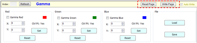
  Figure 15-19: Gamma Read and Write Items

15.7. Shading¶

15.7.1. Adjustment Interface¶

Click on the Shading tree node to call out the ALSC interface on the right-hand side.

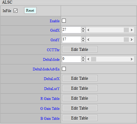
Figure 15-20: Shading Interface

15.7.2. Parameter Description¶

Enable : ALSC API function switch. 0 means disable, and 1 enable. Parameter range: 0 ~ 1.

GridX : X size of shading table. Parameter range: 1 ~ 27. Default is 27.

GridY : Y size of shading table. Parameter range: 1 ~ 17. Default is 17.

CCTThr : Environmental color temperature node setting. This platform supports up to 3 sets of shading table. Note that indexes from small to large need to be filled in the order from low to high color temperature. Parameter range: 1 ~ 3.

DeltaMode : There are 16 preset modes, wherein the vertical axis represents each mode, and the horizontal axis represents the grid size of each grid in the X/Y direction. On this platform, the gride size is X = 26, Y = 16. The larger the value in the preset mode is, the smaller the surrounding grids. Parameter range: 0 ~ 15.

DeltaModeAvdEn : Advanced mode enable switch. 0 means disable, and 1 enable. Parameter range: 0 ~ 1. When GridX/Y is of a size other than the default 27x17 set for this platform, you must enter this mode to do non-equidistant grid settings.

DeltaLutX : X-axis spacing. Each index value represents a block size (index = block size / 16). The index value is limited to 1, 2, 4, 8, and 16. If no block is used, set it to 0. Up to 72 sets of blocks are supported. In this platform, there are 26 blocks.

DeltaLutY : Y-axis spacing. Each index value represents a block size (index = block size / 16). The index value is limited to 1, 2, 4, 8, and 16. If no block is used, set it to 0. Up to 72 sets of blocks are supported. In this platform, there are 16 blocks.

R/G/B Gain Table : Click on any R/G/B gain table, a new interface will be generated. In this platform, the screen is divided into a 27x17 matrix. The value in each box represents the weight by which the R/G/B component at this position needs to be multiplied. Parameter range: 0 ~ 4095.

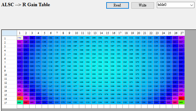
Figure 15-21: Shading 27×17 Table Interface

15.8. Plugin¶

The IQTool provides AF, AWB, CCM, GAMMA and ALSC plugins to aid in IQ tuning, as illustrated in the follpwing Figure.

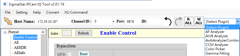
Figure 15-22: Plugin Drop Down Menu

15.8.1. AF Analyzer¶

The AF Analyzer is a plugin tool for auto focus calibration analysis. It utilizes frequency response values to convert filter coefficients.

15.8.1.1. Adjustment Interface

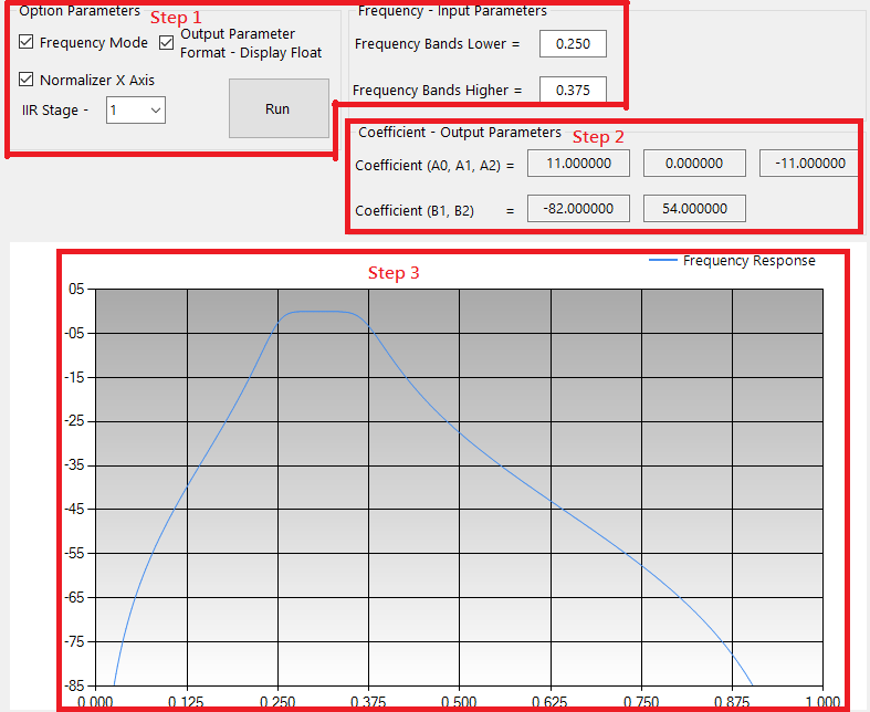
Figure 15-23: AF Analyzer Interface (Frequency Mode)

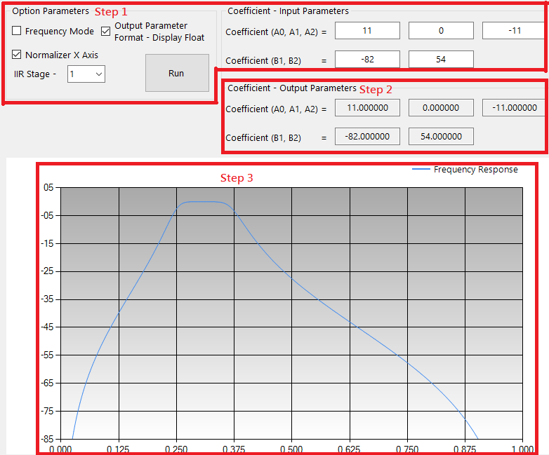
Figure 15-24: AF Analyzer Interface (NonFrequency Mode)

15.8.1.2. Parameter Description

Steps
1. Step 1: Input AF parameter
  
  Frequency Mode: Input the cut-off frequency to produce frequency response.
  
  NonFrequency Mode: Input the AF Fliter coefficient to produce frequency response.
2. Step 2: Output the AF Filter coefficient.
3. Step 3: Output the AF frequency response curve.
Input parameters
1. Bands lower : minimum value of low frequency response, range is 0.001 ~ 1.000.
2. Bands higher : maximum value of high frequency response, range is 0.001 ~ 1.000.
3. Display float option : enable → display AF coefficient; disable → display AF coefficient (2’s complement).
4. Normalizer X-axis option : enable → normalized X-axis value range;
  
  disable → unnormalized X-axis value range.
5. Run button : Calculate coefficients A0, A1, A2, B1, B2 and draw AF frequency response curve.
6. Frequency Mode option : Select the mode for frequency input
7. Coefficient : Input AF Filter coefficients of the various stages when in NonFrequency Mode.
8. IIR Stage : Select the stage for the AF Filter
  
  Frequency Mode: Input the cut-off frequency
  
  NonFrequency Mode: Input the AF Fliter coefficient corresponding to the stage selected. For example, select 1 to input the coefficient of stage 1 AF Filter, and select 2 to input the coefficient of stage 2 AF Filter, and so forth.
Output parameters
1. AF Filter Coefficient: A0, A1, A2, B1, B2
Frequency response curve
1. X-axis: number of sampling points
2. Y-axis: frequency value (db)

15.8.2. AWB Analyzer Combo¶

This plugin tool is used for white balance calibration analysis, and it contains two parts: “Statistics Analyzer” and “Raw Analyzer.” Users can use “Statistics Analyzer” to do color temperature curve ranges calibration, and use “Raw Analyzer” to know the coordinates of each statistic data.

15.8.2.1. Adjustment Interface

Figure 15-25: AWB Analyzer Combo Interface

15.8.2.2. Usage and Parameter Description

Function selection:

Click function tab to select the function.
Statistics source selection:

Click File->Load Statistics on the menu bar. There are three sources for choice.

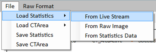
From Live Stream: Statistics from live streaming. Only when IQTool has connected to the camera will this item be available. Users can click “Update Live Statis” button to update the statistics.

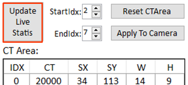
From Raw Image: Statistics from raw image. Please set the raw format on the menu bar before selecting this item.

From Statistics Data: Statistics from statistics file you saved before.
Color temperature ranges source selection:

Click File->Load CTArea on the menu bar. There are two sources for choice.

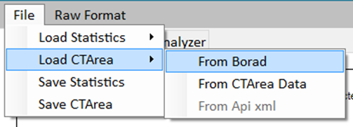
From Board: Get CTArea from the camera. Only when IQTool has connected to the camera will this item be available.

From CTArea Data: CTArea from CTArea file you saved before.
Save statistics: Click File->Save Statistics on the menu bar.
Save color temperature range: Click File->Save CTArea on the menu bar.
Adjust color temperature range:

Directly drag the offset control point (triangle) and range control point (diamond) by mouse.
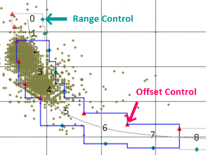
Reset color temperature range: Click “Reset CTArea” button on the upper right.
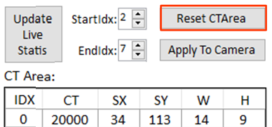
Active color temperature range index:

Set by StartIdx and EndIdx. Only statistics data located on CT blocks with index between StartIdx and EndIdx will be used for calculation.
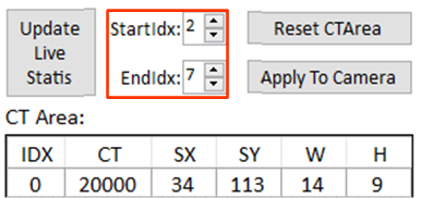
Apply color temperature range: Click “Apply To Camera” button.

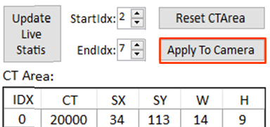
After applying CTArea to camera, be sure to go back to the AWBCTCali page on the IQTool interface and click “Read Page” button (never click “Write Page” before “Read Page”). Only when you do this will the adjusted color temperature range be saved alongwith API bin file.
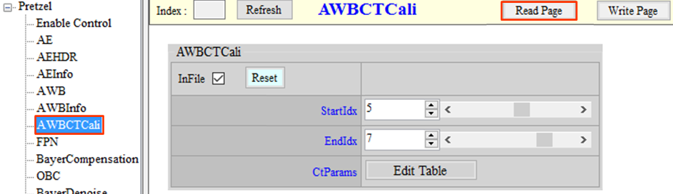
Move & scale the raw image:

Directly drag the image by left key of the mouse to move the image position.

Scroll up or down the mouse wheel to zoom in or out.
Show statistics blocks: Check “Show Statistics Blocks,” then the statistics blocks will be shown on image.
Select statistics block: Double click left key of the mouse, then the statistics block will be selected. The statistics information will be shown in the “statistics info” box on the left. Besides, the coordinate of the block (Star) will also be shown on the R/G - B/G coordinate plane. Click right key of the mouse to cancel the selection.
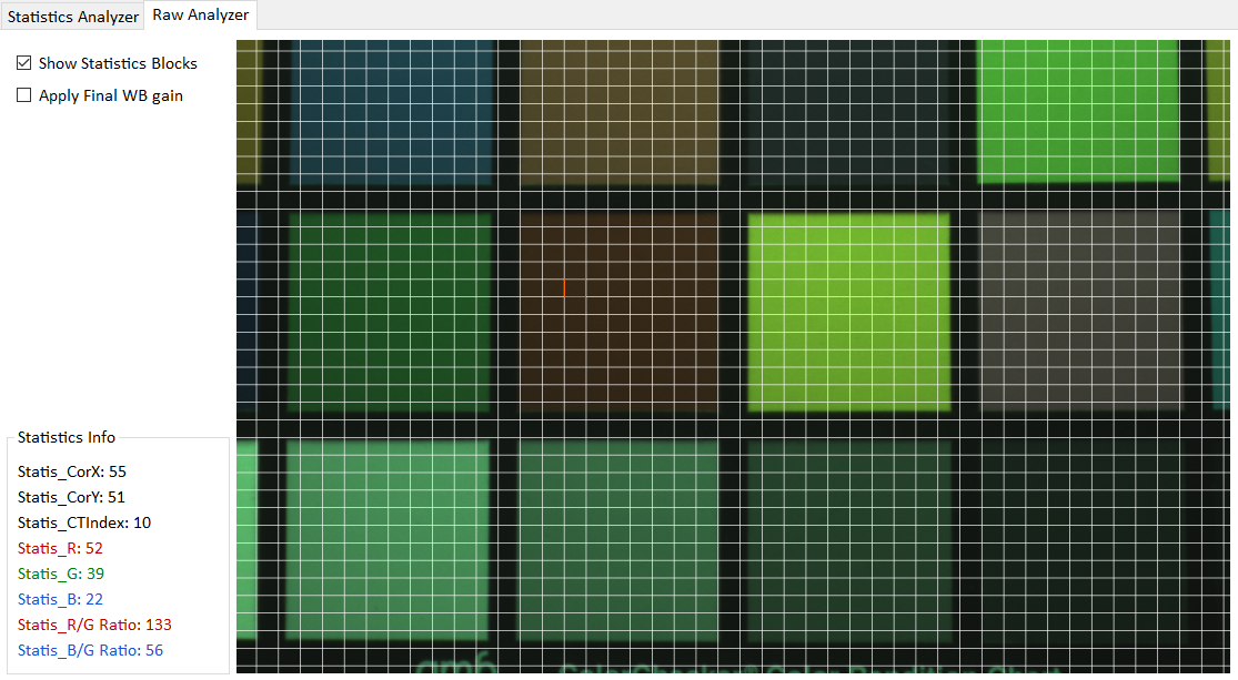
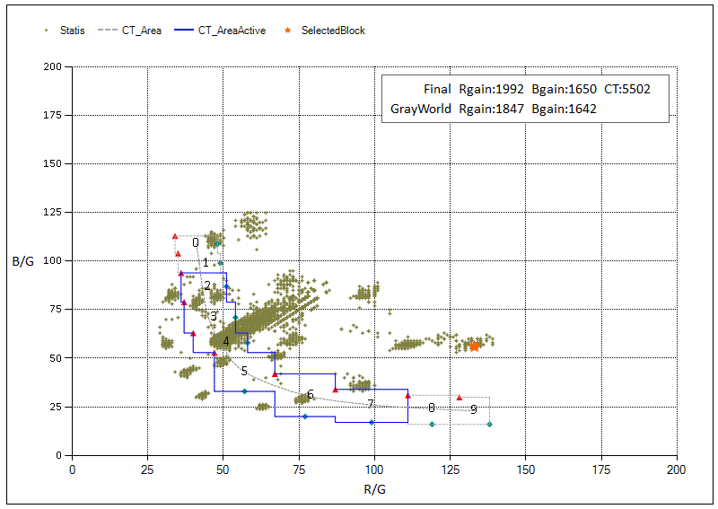
Show applied Final RBgain image: Check “Apply Final WB gain.”

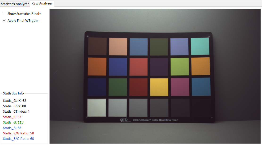
15.8.3. CCM Analyzer¶

This plugin tool is used for color correction.

15.8.3.1. Adjustment Interface

Calculate CCM page is used for CCM calibration. It will read reference values from the camera when activated. Before launching CCM Analyzer, you will have to fill in the correct data to the manual sections of both Gamma and OBC; hence, offline tuning is not supported. The other page, FineTuneMatrix, is for fine-tuning.

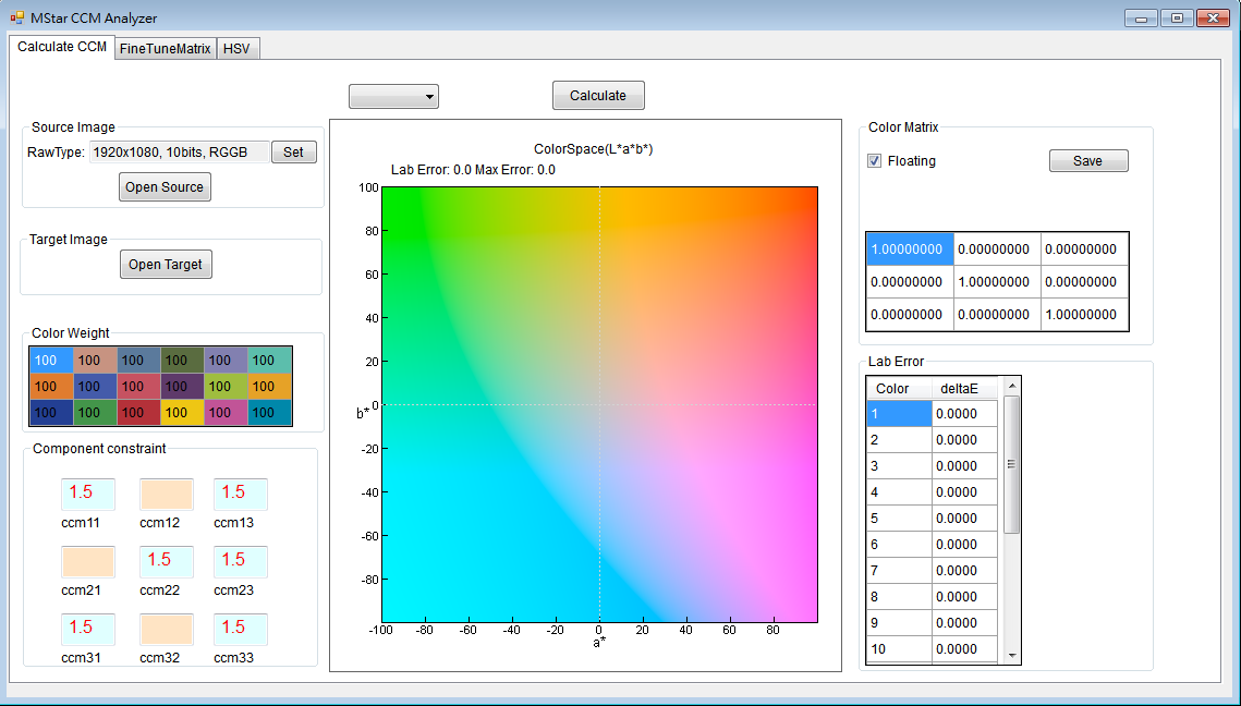
Figure 15-26: CCM Analyzer Interface

15.8.3.2. Usage and Parameter Description

Usage

Click on the Set button from Source Image to set the raw data. Click on the Open Source button to load saved raw image. When the selected source is opened, a window with the raw image will be shown. Drag your mouse directly on the screen to ensure that all color blocks have been checked, then click OK. Click on the Open Target button from Target Image to open the standard color checker image and select the color checker in the same way mentioned above.

Figure 15-27: Load Raw Image Window Interface
Parameter Description
- Color Weight:
  
  Allows you to adjust the weight of each color block. Color blocks with greater weight will achieve more accurate fitting result. Default value is 100.
  
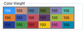
  Figure 15-28: Color Weight Setting Interface
- Component Constraint:
  
  Allows you to set a constraint against any component, where necessary; for example, if you set a constraint of 0.5 to some component, then the fitting result of that component will be limited to the range from -0.5 to 0.5.
  
  Figure 15-29: Component Constraint Setting Interface
- Once set, click on the “Calculate” button and the final fitting result will be shown at the right side of the interface.
  
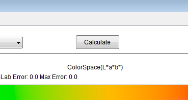
  Figure 15-30 : CCM Interface
- Repeat the foregoing step to generate the color matrix of the remaining color temperatures.

15.8.4. Gamma Fitting Analyzer¶

This plugin tool is used for Gamma fitting calibration.

15.8.4.1. Adjustment Interface

CDF_Orig : The CDF curve from Open Source

CDF_Ref : The CDF curve from Open Target

FitGMA : Fitting Gamma curve

Figure 15-31: Gamma Fitting Analyzer Interface

15.8.4.2. Usage and Parameter Description

Usage
1. Read the Gamma curve of the image and select Raw Setting from Options.
  
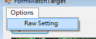
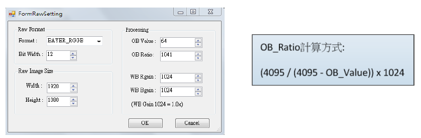
  Figure 15-32: Opening Raw Setting Interface
2. Click on the Open Source button to load saved raw image.
3. Click on the Open Target button to open a standard OECF Chart image.
4. Left-click to select the ROI to generate the corresponding histogram automatically.
5. Select Gamma curve type. There are two types for curve calculation. We suggest that you select Exponential.
  - Spline curve
  - Exponential curve
6. Click on the Match GMA button to generate the Gamma curve.
7. Press the Save GMA button to save the final Gamma parameters.

15.8.5. SstarCalibration Tool¶

This plugin tool is used for shading and black level calibration. The functions are identical with those available from the calibration tool.

15.8.5.1. CalibrationALSC Adjustment Interface

Please refer to the figure below for the CalibrationALSC adjustment interface.

Figure 15-33: CalibrationALSC Interface

15.8.5.2. Usage and Parameter Description

Parameter setting
- Ratio Table: Picture center to corner correction intensity ratio. Parameter range: 0 ~ 255.
This parameter allows you to adjust the weight of each color block. The higher the weight, the more accurate the fitting result is. Default value is 100.
- OBC: The OB value of current sensor in 16-bit. Parameter range: 0 ~ 65535.
- GridX, GridY: Size of shading table.
- Set Delta Format: Non-isometric block setting.
  1. Delta Mode: 16 modes are provided by default. Parameter range: 0 ~ 15. For details on the setting method, see Figure 16-6 and Figure 16-7.
  2. Delta Mode Advance Enable: Advance mode enable switch. 0 means disable, 1 enable. Parameter range: 0 ~ 1. When GridX/Y is of a size other than the default set for this platform, you must enter this mode to do non-equidistant grid settings.
  3. Delta X Lut: X-axis spacing. The actual number of pixels is the value multiplied by 16. Only 1, 2, 4, 8, and 16 are valid values. For unused blocks, set it to 0.
  4. Delat Y Lut: Y-axis spacing. The actual number of pixels is the value multiplied by 16. Only 1, 2, 4, 8, and 16 are valid values. For unused blocks, set it to 0.
- CT: Color temperature. Parameter range: 1 ~ 20000.
- CT Num: Chooses the number of sets of color temperate table data to be corrected, the default is to correct 3 sets of color temperature table. Parameter range: 1 ~ 3.
- CT Index: Selects which group of tables is to be calibrated. Up to 3 groups are supported. The calibration sequence does not need to follow the order of 0 to 2. However, it is necessary to ensure that the environmental color temperatures of 0 to 2 go from low to high and are not the same.
- Open Raw Image: Selects the path of raw image.
- Set Raw Format: Sets the raw image related parameters.
- Apply Demosaicing: Applies a simple demosaic process to the raw image.
- Show Alsc Table: Shows the shading table.
- Color: Shows the shading table R/G/B gain.
- GenTable: Generates shading table according to the parameter entered.
- ApiApply: Only the shading table of the current CT index will be downloaded to the API.
- CaliApply: Transfers all parameters to the EVB at once according to the current size of CTNum.
- Debug Log: Shows the debug log when using GenTable and Apply parameters.
- Keep Cali Data: Loads the generated .data file so that the previous results can be retained and continue to be corrected.
- Dump Data: Generates a txt file of correction results.
- Load Cali Data: Loads the generated .data file so that it can be used with CaliApply to apply the correction result of that .data.
- Select Cali File: Clickable only when “Load Cali Data” is checked and for the purpose of selecting .data file to be set on the EVB board.
Usage

There are two routes depending on whether “Load Cali Data” is checked:

(a) Checked
1. After checking “Load Cali Data,” click “Select Cali Data” and select the .data you want to apply.
2. After selecting the desired .data, only CaliApply can be used.
At this time, the calibration parameters being applied will not be displayed on our SStarCalibration Tool.

(b) Unchecked
1. Click “Set Raw Format” to set the raw image information, and click “Open Raw Image” to open the raw image. You can check “Apply Demosaicing” to see the RGB image. This is just a simple demosaic function, which is different from the actual one. Whenever “Load Cali Data” changes from checked to unchecked, you need to click “Open Raw Image” to open the raw image again.
2. Set the parameters for generating shading table, including Ratio Table, OBC, GridX, GridY, Set Delta Format, and then click “GenTable” to generate shading table. You can check “Show Alsc Table” to see the shading table. If you want to keep the results and continue after finishing calibrating the first set of parameters, you can check “Keep Cali Data.” Note: If the size of CT Num has been changed when you calibrate the second set of parameters, the Keep Cali Data function will be lost.
3. Set the parameters down to the board, including CT and CT Index, and then click ApiApply or CaliApply to put them into effect. Be sure to go to the ALSC interface and click “Read” to see the same parameters as CalibrationALSC. Upon the completion of each Apply, GenTable, CaliApply and ApiApply will be grayed out. At this time, any change to the settings in the red frame as shown in the figure above will allow you to recalibrate again.

15.8.5.3. CalibrationLSC Adjustment Interface

Please refer to the figure below for the CalibrationLSC adjustment interface.

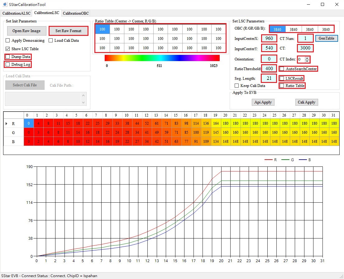
Figure 15-34: CalibrationLSC Interface

15.8.5.4. Usage and Parameter Description of CalibrationLSC Interface

Parameter setting
- Ratio Table: Picture center to corner correction intensity ratio. Parameter range: 0 ~ 255.
This parameter allows you to adjust the weight of each color block. The higher the weight, the more accurate the fitting result is. Default value is 100.
- OBC: The OB value of current sensor in 16-bit. Parameter range: 0 ~ 65535.
- InputCenterX, InputCenterY: Sets the position of the image’s brightest center point. Parameter range: 0 ~ 4095.
- CT: Color temperature. Parameter range: 1 ~ 20000.
- CT Num: Selects which group of tables is to be calibrated. Up to 3 groups are supported. The calibration sequence does not need to follow the order of 0 to 2. However, it is necessary to ensure that the environmental color temperatures of 0 to 2 go from low to high and are not the same.
- CT Index: It supports up to 3 sets of color temperature, the parameter range is 0 ~ 2. The index will be linked according to the size of CTNum.
- Open Raw Image: Selects the path of raw image.
- Set Raw Format: Sets parameters related to the raw image.
- Apply Demosaicing: Applies a simple demosaic process to the raw image.
- Show LSC Table: Shows the shading table.
- GenTable: Generates shading table according to the parameter entered.
- ApiApply: Only downloads the shading table of the current CT index to the API.
- CaliApply: Transfers all parameters to the EVB at once according to the current size of CTNum.
- Debug Log: Shows the debug log when using GenTable and Apply parameters.
- Keep Cali Data: Loads the generated .data file so that the previous results can be retained and continue to be corrected.
- Dump Data: Generates a txt file of correction results.
- Load Cali Data: Loads the generated .data so that it can be used with CaliApply to apply the correction result of that .data.
- Select Cali File: Clickable only when “Load Cali Data” is checked and for the purpose of selecting .data to be set on the EVB board.
- Orientation: Sets the sampling point direction, from the brightest center point of the image to corner point. 0: upper-left, 1: upper-right, 2: lower-right, 3: lower-left
- Seg. Length: Cuts the length and distance of the sampling point.
- AutoSearchCenter: Selects to automatically detect the brightest center position of the input image. Parameter range: 0 ~ 1, recommended to set 1.
- LSCResult: Dumps LSC result image.
- Ratio Table: Whether to use the compensation value of the Ratio Table to correct. The Ratio Table can only be changed when this item is checked.
- RatioThreshold: It is used to avoid over-compensation of vignetting. Larger value means that there is more vignetting compensation, and smaller value represents less compensation. More vignetting compensation will cause the normal data close to the corner to be over compensated. When the threshold is smaller, the compensation value will be found according to the current maximum index value, and then set to the maximum value, while the index value after the maximum index value maintains the maximum compensation value (without increasing the value); the larger the threshold is, the larger will the compensation value become. Ratio Base: 100; parameter range: 0 ~ 25600.
Usage

There are two routes depending on whether “Load Cali Data” is checked:

(a) Checked
1. After checking “Load Cali Data,” click “Select Cali Data” and select the .data you want to apply.
2. After selecting the desired .data, only “CaliApply” can be used.
  
  At this time, the calibration parameters being applied will not be displayed on our SStarCalibration Tool.
(b) Unchecked
1. Click “Set Raw Format” to set the raw image information, and click “Open Raw Image” to open the raw image. You can check “Apply Demosaicing” to see the RGB image. This is just a simple Demosaic function, which is different from the actual one. Whenever “Load Cali Data” changes from checked to unchecked, you need to click “Open Raw Image” again to open the raw image.
2. Set the parameters for generating shading table, including Ratio Table, OBC, InputCenterX, InputCenterY, and then click “GenTable” to generate shading table. You can check “Show LSC Table” to see the shading table. If you want to keep the results and continue after finishing calibrating the first set of parameters, you can check “Keep Cali Data.” Note: If the size of CT Num has been changed when you calibrate the second set of parameters, the Keep Cali Data function will be lost.
3. Set the parameters down to the board, including CT and CT Index, and then click “ApiApply” or “CaliApply” to put them into effect. Be sure to go to the LSC interface and click “Read” to see the same parameters as “CalibrationLSC.” Upon the completion of each Apply, GenTable, CaliApply and ApiApply will be grayed out. At this time, any change to the settings in the red frame as shown in the figure above will allow you to recalibrate again.

15.8.5.5. CalibrationOBC Adjustment Interface

Please refer to the figure below for the CalibrationOBC Adjustment Interface.

Figure 15-35: CalibrationOBC Interface

15.8.5.6. Usage and Parameter Description

Parameter setting
- Open Raw Image: Selects the path of raw image.
- Set Raw Format: Sets the raw image related parameters.
- Apply Demosaicing: Applies a simple demosaic process to the raw image.
- Show OBC Table: Shows the shading table after OBC calibration.
- CalOBGain: Generates the value of the corrected black current according to the input parameters.
- ApiApply: Puts the calibration result on the board.
- CaliApply: Puts the calibration result on the board.
- Debug Log: Shows the debug log when using CalOBGain and Apply parameters.
- Keep Cali Data: Loads the generated .data file so that the previous results can be retained and continue to be corrected.
- Dump Data: Generates a txt file of correction results.
- Load Cali Data: Loads the generated .data so that it can be used with CaliApply to apply the correction result of that .data.
- Select Cali File: Clickable only when “Load Cali Data” is checked and for the purpose of selecting .data to be set on the EVB board.
- Weight Table: Divides the picture into 3 $<span><span class="MathJax_Preview">\times</span><script type="math/tex">\times$ 3 blocks. The weight of each block is 0 to 16 when calculating the OB and is recommended to set 1.
- AutoAssign: Sets the OB value to all Gain, the value range is 0 ~ 1. It is recommended to set 1.
- Cali Gain Index: Selects which group of OB values to calibrate, the value range is 0 ~ 15.
- SetOBCParameters-Weight Table: Displays the Weight Table.
- Target: The desired residual value after correction in 16-bit. The value range is 0 ~ 65535, and it is recommended to set 0.
Usage

There are two routes depending on whether “Load Cali Data” is checked:

(a) Checked
1. After checking “Load Cali Data,” click “Select Cali Data” and select the .data you want to apply.
2. After selecting the desired .data, only CaliApply can be used.
At this time, the calibration parameters being applied will not be displayed on our SstarCalibration Tool.

(b) Unchecked
1. Click “Set Raw Format” to set the raw image information, and click “Open Raw Image” to open the raw image. You can check “Apply Demosaicing” to see the RGB image. This is just a simple Demosaic function, which is different from the actual one. Whenever “Load Cali Data” changes from checked to unchecked, you need to click “Open Raw Image” again to open the raw image.
2. Set the parameters for generating table, including Weight Table, Target, AutoAssign, Cali Gain Index, and then click CalOBGain to generate table. You can check Show OBC Table to see the table. If you want to keep the results and continue after finishing calibrating the first set of parameters, you can check “Keep Cali Data.”
3. Set the parameters down to the board then click ApiApply or CaliApply to put them into effect. Be sure to go to the ALSC interface and click “Read” to see the same parameters as CalibrationALSC. Upon the completion of each Apply, GenTable, CaliApply and ApiApply will be grayed out. At this time, any change to the settings in the red frame as shown in the figure above will allow you to recalibrate again.

15.8.5.7. Raw Setting Parameter Interface

Please refer to the figure below for the Raw Setting Parameter Interface.

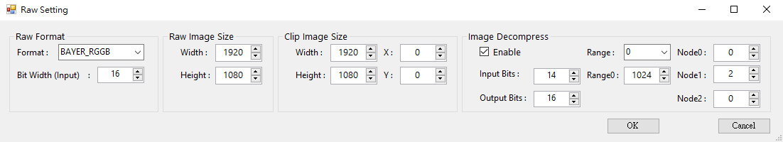
Figure 15-36: Raw Setting Interface

15.8.5.8. Raw Setting Parameter Description

Raw Format
- Format: Raw image RGB format.
- Bit Width (Input): Raw image input bit.
Raw Image Size
- Width: Raw image width.
- Height: Raw image height.
Clip Image Size
- Width: The width of the raw image after Clip.
- Height: The height of the raw image after Clip.
- X: Raw image to be clipped from the width. Note that the starting position plus the size of the clip you want cannot exceed the size of Raw image.
- Y: Raw image to be clipped from the height. Note that the starting position plus the size of the clip you want cannot exceed the size of Raw image.
Image Decompress
- Enable: Whether to turn on the Decompress function.
- Input Bits: Compressed bits.
- Output Bits: Decompressed bits.
- Range: There are four intervals to be set.
  - Range0: Set the first interval, 0 ~ Range0.
  - Range1: Set the second interval, Range0 ~ Range1.
  - Range2: Set the third interval, Range1 ~ Range2.
  - Range3: No need to set the fourth interval, Range2 ~ ∞.
- Node0: Offset of the corresponding interval.
- Node1: Shift of the corresponding interval.
- Node2: Base of the corresponding interval.

16. CALIBRATION TOOL¶

The calibration tool supports OBC, ALSC, LSC and AWB production line correction. As additional offline calibration tool is required, please make sure that redistributable packages for Visual Studio 20xx have been successfully installed to the operating environment (Link:x86, x64).

16.1. Calibration Flow¶

Grab the Raw image under various scenarios, set the parameters (by modifying *.ini), generate *.data, and then burn the *.data in.

16.1.1. Grabbing Raw Image¶

16.1.2. Parameter Description¶

Set up the environmental parameters at the path: calibration\SampleCode\Release\CalibrationInitialParameter.ini.

[RAW_INFO]

filename : Filename of the Raw image.

The raw data follows the naming rule of “filename” + “_” + “three numbers”
frame_numbers : Number of Raw images in single calibration, normally 1, except for SDC, which often calibrates multiple frames at a time.
frame_start_index : Raw image index.
- If filename = "SDC" and frame_start_index = 1, the Raw image in sample code should be named as SDC_001.
- If three frames of Raw image are required for calibration, filename = "SDC," frame_start_index = 2, frame_numbers = 3, then the Raw image should be named as SDC_002, SDC_003, and SDC_004.
width : Raw image width.
height : Raw image height.
clip_x : Starting X coordinate of the clip image. To avoid Bayer Pattern disorder, we suggest setting an even number.
clip_y : Starting Y coordinate of the clip image. To avoid Bayer Pattern disorder, we suggest setting an even number.
clip_width : Clip image width. To avoid Bayer Pattern disorder, we suggest setting an even number.
clip_height : Clip image height. To avoid Bayer Pattern disorder, we suggest setting an even number.
dump_clip_image : Enable/disable dump clip image function. 0 means disable, and 1 enable. Default is 0.
cfa_type : Bayer pattern sequencing, i.e. the color block on the top left corner.

[0 = RGGB, 1 = GRBG, 2 = BGGR, 3 = GBRG]
source_type : 0 for Raw; modification not suggested.
in_data_precision : Precision of the input Raw image, default is 16.
out_data_precision : Precision of the output *.data, default is 16.
cali_output_path : Output path; modification not suggested.

[CALI_INFO]

calibration_select : Calibration item: AWB = 0, OBC = 1, SDC = 2, ALSC = 3, LSC = 4.
load_calibration_data : Load *.data. Must be set to 0 for the first calibration, and 1 for the subsequent calibration(s), if any, so that the previous calibration data can be saved. This parameter is often used for OBC, ALSC, LSC, AWB and SDC. Note that This platform does not support SDC feature.
load_calibration_data : Twinkie = 2, Pretzel = 3, Macaron = 4, Pudding = 5, Ispahan = 6, Ikayaki = 7, Mercury5 = 16, Tiramisu = 17.

[CALI_DB]

cali_dump_data : Switch for Dump .txt file. 0 only generates *.data file, and 1 will generate *.txt in addition to *.data file.
cali_xxx_xxx_path : Path for the *.data after calibration; modification not suggested.

[OBC] [ALSC] [LSC] [AWB] : As described in the subsequent section.

16.1.3. Generating *.data¶

Place the raw image for calibration under calibration\SampleCode\Release\image.
Modify calibration\SampleCode\Release\CalibrationInitialParameter.ini.

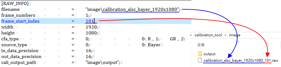
Figure 16-1: CalibrationInitialParameter.ini - RAW_INFO Parameters Setting Description
Execute calibration\SampleCode\Release\CalibrationRelease.exe.
The calibration flow will check the execution path to make sure the data and image folders have been automatically created under calibration folder successfully.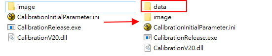

Figure 16-2: Checking Data Folder Required for Calibration
If the calibration turns out successful, you can find the calibration *.data from calibration\SampleCode\Release\data\cfg.

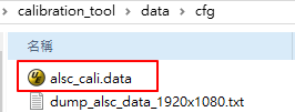
Figure 16-3: Generating *.data File Required for Calibration

16.1.4. Burning *.data¶

Place *.data at the directory DownloadTool_XXX\FactRes\ and re-burn.

NOTE: Do NOT change the *.data filename.

16.2. OBC Adjustment¶

OB adjustment is used to calibrate the black level of the sensor.

16.2.1. Calibration Environment¶

The calibration must be done under a dark environment, with all available light sources blocked out. When darkening the environment, watch the streaming video closely to see if there is any abnormality. Go to the next step if nothing unusual happens. Stop the calibration and report the issue if something abnormal is found; resume after the issue is resolved.

Figure 16-4: Example of Abnormal OB Dark Screen

16.2.2. Parameter Description¶

AutoAssign : Automatically assign an OB value to all gains. Parameter range: 0~ 1. Suggested value is 1.

Target : The expected residual value after calibration in 16-bit. Parameter range: 0 ~ 65535. Suggested value is 0.

Weight : The weight of each of the 3×3 blocks into which the screen is equally divided for OB calculation. Parameter range: 0 ~ 16. We suggest setting all blocks to 1.

CaliGainIndex : Fills in values according to ISO index. Parameter range: 0 ~ 15.

16.2.3. Calibration Steps¶

Set the total gain to the smallest possible gain and grab the Raw image under darkened environment.
If the mode is normal mode or combine mode, set “out_data_precision” to 16.
Generate obc_cali.data or dump_obc_data.txt if you would like to view the calibration result, and then load the obc_cali.data.
If the mode is normal mode or combine mode, the OB value in 16-bit will be inputted to the blacklevel in the OBC interface over the IQTool.
If the mode is HDR mode, short exposure and long exposure should be calibrated separately.
- Short exposure calibration: As in normal mode, grab the Raw image under darkened environment using short exposure setting, set “out_data_precision” to 16, generate obc_cali.data, and then load obc_cali.data. The OB value in 16-bit will then be inputted to the blacklevel in the OBC interface over the IQTool.
- Long exposure calibration: Grab the Raw image under darkened environment using long exposure setting, set “out_data_precision” to 16, generate dump_obc_data.txt, and then manually input the value to the blacklevel_1 in the OBC interface over the IQTool in 16-bit.

Note:

Normal mode : including Linear mode (single frame) and HDR mode (2 frames).
Combine mode : the composite image after sensor completes long and short exposure calibration, including image file compression program.

16.2.4. Precautions¶

If the difference between high gain and low gain in OB is so large that you need to set different OB to different ISO index, use the AE to manually set the respective ISO index gains. Grab the Raw image under darkened environment, generate the dump_obc_data.txt, and then manually input the value to the 16 nodes of the blacklevel Auto Mode in the OBC interface over the IQTool.

16.3. ALSC Adjustment¶

Since different combinations of lens and sensor lead to different Y shading and color shading, it is best to evaluate if ALSC calibration is required whenever the lens or sensor has been replaced.

ALSC calibration will generate a 27 x 17 table for R, G and B respectively, with different R, G and B gain allotted to different screen regions, and will therefore help improve both Y shading and color shading. ALSC calibration supports up to three color temperatures, but table interpolation is not supported.

16.3.1. Calibration Environment¶

The calibration environment requires a uniform light source, preferably using a Macbeth standard light booth along with a diffuser. In the absence of a diffuser, try calibrate the ALSC against the gray wall within the light booth to make the light as uniform as possible.

Before calibration, make sure that OB and AWB color temperature curve ranges have both been calibrated and correctly applied. Moreover, when using the RGB sensor, see to it that the IR cut is well caped.

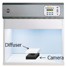
Figure 16-5: LSC/ALSC Calibration Environment Setup Example

16.3.2. Parameter Description¶

TargetIndex : Selects which table is to be calibrated. Up to three tables can be calibrated at the same time. Calibration process does not have to follow the sequence from 0 to 2; all you have to do is to make sure the environmental color temperatures of 0 to 2 go from low to high.

CCTNumber : Chooses the total number of sets of color temperate table data to be corrected, the default is to correct 3 sets of color temperature table. Parameter range: 1 ~ 3.

GridX/Y : Size of shading table. This platform is set to 27x17 by default.

GridNumMax : Max size of shading table, which is a fixed number. GridNumMax of this platform is 27x17=459.

Segment_Delta_Str_Mode : There are 16 preset modes, wherein the vertical axis represents each mode, and the horizontal axis represents the grid size of each grid in the X/Y direction. On this platform, the gride size is X = 26, Y = 16. The larger the value in the preset mode is, the smaller the surrounding grids. Parameter range: 0 ~ 15.

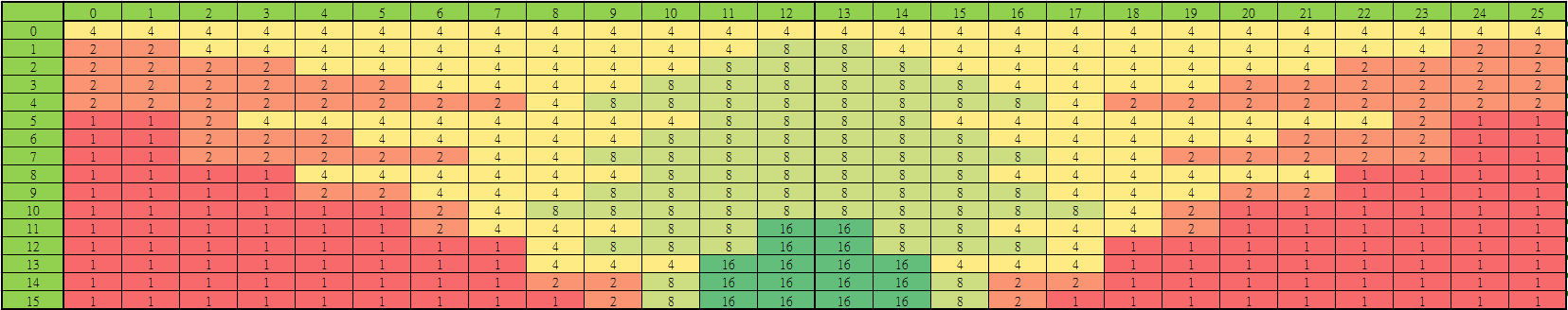
Figure 16-6: Distribution of the 16 Default Modes for Delta_LUT_X

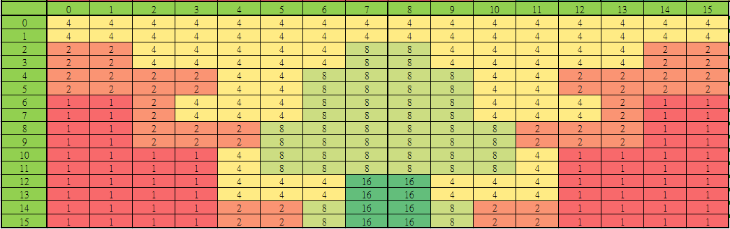
Figure 16-7: Distribution of the 16 Default Modes for Delta_LUT_Y

ColorTemperature : Environmental color temperature of the current TargetIndex.

OB_R/G/B_Value : OB value of current sensor. Parameter range is 0 ~ 65535 (in 16-bit).

RatioTable_R/G/B`Num’ : Screen center to corner correction intensity ratio. Parameter range is 0 ~ 255.
NOTE: ‘Num’ refers to the number of values, 0 for center, and 8 for the four corners.

UnitGainResult : Selects whether to generate 1x gain Shading Table. 0 means disable, 1 enable. Parameter range: 0 ~ 1.

PortraitEnable : Checks the width and height of an image. 0 means disable, 1 enable. Parameter range: 0 ~ 1.

Segment_Delta_Adv_Enable : Switch to enable/disable advance mode. 0 means disable, 1 enable. Parameter range: 0 ~ 1. When GridX/Y is of a size other than the default 27x17 set for this platform, you must enter this mode to do non-equidistant grid settings.

Segment_Delta_LUT_X0 ~ 8 : X-axis spacing. Each 4 bits represent an index value [index = (block size / 16) - 1]. So the actual number of pixels = (index + 1) x 16. The index value is limited to 1, 2, 4, 8, and 16. If no block is used, set it to 0. Up to 72 sets of blocks are supported. In this platform, there are 26 blocks.

Segment_Delta_LUT_Y0 ~ 8 : Y-axis spacing. Each 4 bits represent an index value [index = (block size / 16) - 1]. So the actual number of pixels = (index + 1) x 16. The index value is limited to 1, 2, 4, 8, and 16. If any block is not used, set it to 0. Up to 72 sets of blocks are supported. In this platform, there are 16 blocks.

16.3.3. Calibration Steps¶

Decide the number of light sources to be calibrated. Set the AE target to about 1500 and capture raw data of each color temperature. Make sure raw data are not overexposed, and move them to the “image” folder in calibration tool path. Note: AE target data range = 10 ~ 2550.
Open CalibrationInitialParameter.ini file and set parameters of [RAW INFO] section.

(Please refer to Section 16.1.2.)
- Select file path and format of raw data.
- Set in/out_data_precision to 16.
- Set calibration_select to 4.
- Set load_calibration_data to 0 for first calibration; set to 1 for remaining calibrations.
Set parameters of [ALSC] section in CalibrationInitialParameter.ini file. (Please refer to Section 16.3.2.)
Execute CalibrationRelease.exe to create alsc_cali.data.
Repeat Steps 2 to 4 to complete ALSC calibration for all color temperature light sources to get the final alsc_cali.data. If cali_dump_data in [CALI_DB] section is set to 1, a dump_alsc_data.txt file will also be created after calibration. You can check the shading table in this txt file.
Use MI_ISP_API_CmdLoadCaliDat API to apply alsc_cali.data.

(Please refer to SStar_PUDDING_ISP_Software_Development_Guide for details.)

16.3.4. Adjustment Interface¶

Select “Shading” from the menu on the left-hand side to find the ALSC and ALSC_CTRL adjustment interface.

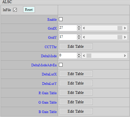
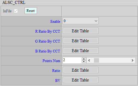
Figure 16-8: ALSC and ALSC_CTRL Adjustment Interface

16.3.5. Parameter Description¶

R Gain Table : ALSC R table. Parameter range is 0 ~ 8191.

G Gain Table : ALSC G table. Parameter range is 0 ~ 8191.

B Gain Table : ALSC B table. Parameter range is 0 ~ 8191.

R Ratio By CCT : ALSC table total R ratio (128 = 1x). Parameter range is 0 ~ 128.

G Ratio By CCT : ALSC table total G ratio (128 = 1x). Parameter range is 0 ~ 128.

B Ratio By CCT : ALSC table total B ratio (128 = 1x). Parameter range is 0 ~ 128.

Points Num : Number of point for Ratio by BV (Different Ratio can be set according to different ambient brightness values [BV]).

Ratio : Ratio at each point.

BV : BV value corresponding to to each point.

16.3.6. Adjustment Steps¶

Tune Ratio by BV. Generally, the ratio is reduced under low BV, which can alleviate the noise in the outside area.
Tune the R/G/B Ratio By CCT, which is set to 1x originally, if necessary.

16.3.7. Precautions¶

ALSC R/G/B Gain table is saved in both iqfile and alsc_cali.data, but the table can only be read/written in API bin. The table cannot be saved in API bin due to size limitation. As a result, you needs to load alsc_cali.data every time when booted up.

16.3.8. .data Format and Size¶

Handle size : 20 bytes

Ctrl size : 52 bytes

Data size : 4 + x bytes; x = the value of [(GridX * GridY * 3 * 2 + 2 * GridMax) / 4] rounding to the nearest one and then multiplying by the larger sum between 4 GridMax = GridX or GridY

Total size : 20 + 52 * cctNum + (4 + x) * cctNum bytes; cctNum = the number of sets of color temperate for calibration (1 ~ 3)

16.4. LSC Adjustment¶

LSC calibration will generate a table of 32 for each of R, G and B, with different R, G and B gains allotted to different screen region, and will therefore help improve Y shading. LSC calibration supports up to three color temperatures, but table interpolation is not supported.

16.4.1. Calibration Environment¶

Same as ALSC.

16.4.2. Parameter Description¶

TargetIndex : Selects which table is to be calibrated. Up to three tables can be calibrated at the same time. Calibration process does not have to follow the sequence from 0 to 2; all you have to do is to make sure the environmental color temperatures of 0 to 2 go from low to high.

CCTNumber : Chooses the number of sets of color temperate table data to be corrected, the default is to correct 3 sets of color temperature table. Parameter range: 1 ~ 3.

TableSize : Size of shading table, default is 32. Modification is not suggested.

LSCResult : Dumps LSC result image.

SegmentLength : Segments the sampling length.

AutoCenter : Detects the brightest point automatically. Parameter range is 0 ~ 1, suggested value is 1. If 0, InputOrientation and InputCenterX/Y can be used for manual setting.

InputOrientation : Sets sampling direction from the brightest center point to the corner. 0: Upper-left; 1: Upper-right; 2: Lower-right; 3: Lower-left.

InputCenterX/Y : Location of the brightest point. Parameter range is 0 ~ 4095.

ColorTemperature : Environmental color temperature of current TargetIndex.

OB_R/G/B_Value : OB value of current sensor. Parameter range is 0 ~ 65535 (in 16-bit).

RatioTable_R/G/B’Num’ : Screen center to corner correction intensity ratio. Parameter range is 0 ~ 255. NOTE: ‘Num’ refers to the number of values. Parameter range: 0 ~ 8.

Ratio_Threshold : Used to avoid over-compensation of vignetting. Larger value means that there is more vignetting compensation, and smaller value represents less compensation. More vignetting compensation will cause the normal data close to the corner to be over compensated. When the threshold is smaller, the compensation value will be found according to the current maximum index value, and then set to the maximum value, while the index value after the maximum index value maintains the maximum compensation value (without increasing the value); the larger the threshold is, the larger will the compensation value become. Ratio Base: 100; parameter range: 0 ~ 25600.

DebugLSCInfo : For debug mode only. This parameter will provide the related error messages to SigmaStar for problem analysis. 0 means disable, 1 enable. Parameter range: 0 ~ 1. Suggested setting is 0.

16.4.3. Calibration Steps¶

Same as ALSC.
Generate lsc_cali.data. You can also generate dump_lsc_data.txt or dump_lsc_result.raw to view the calibration result, and then load lsc_cali.data. Skip this step if LSC calibration is not performed.

16.4.4. Adjustment Interface¶

The LSC and LSC_CTRL interfaces appear when you click on Shading from the menu on the left-hand side.

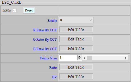
Figure 16-9: LSC and LSC_CTRL Adjustment Interface

16.4.5. Parameter Description¶

R Gain Table : LSC R table. Parameter range is 0 ~ 1023.

G Gain Table : LSC G table. Parameter range is 0 ~ 1023.

B Gain Table : LSC B table. Parameter range is 0 ~ 1023.

R Ratio By CCT : LSC table addtional R ratio (128 = 1x). Parameter range is 0 ~ 128.

G Ratio By CCT : LSC table addtional G ratio (128 = 1x). Parameter range is 0 ~ 128.

B Ratio By CCT : LSC table addtional B ratio (128 = 1x). Parameter range is 0 ~128.

Points Num : Number of point for Ratio by BV (Different Ratio can be set according to different ambient brightness values [BV]).

Ratio : Ratio at each point.

BV : BV value corresponding to each point.

16.4.6. Adjustment Steps¶

Tune Ratio by BV. Generally, the ratio is reduced under low BV, which can alleviate the noise caused by LSC in the outside area.
R/G/B Ratio By CCT is set to 1x as default; tune it if necessary.
If necessary, tune R/G/B Gain table directly.

16.4.7. Precautions¶

LSC R/G/B Gain table exists in iqfile, lsc_cali.data and API bin at the same time. The values in iqfile will be taken as the default values, and replaced by API bin, and then lsc_cali.data, if any.
The normal flow is to load lsc_cali.data instead of the API bin, so that the R/G/B Gain table will be stored in API bin. This way, you can do the tuning over the API bin directly, without loading lsc_cali.data every time.

16.4.8. .data Format and Size¶

Handle size : 20 bytes

Ctrl size : 60 bytes

Data size : 8 + x bytes; x = the value of [(2 + TableSize * 3 * 2) / 4] rounding to the nearest one and then multiplying by 4.

Total size : 20 + 60 * cctNum + (8 + x) * cctNum bytes; cctNum = the number of sets of color temperate for calibration (1 ~ 3)

16.5. AWB Adjustment¶

AWB is used for production line calibration, to compensate for the statistical difference in white balance between different camera modules and the golden sample.

16.5.1. Calibration Environment¶

Place a gray card in the light booth and grab the Raw data with the gray card occupying the whole picture.

16.5.2. Parameter Description¶

CaliState : Selects calibration mode.

0 represents CALIB_GOLDEN_H; 1 represents CALIB_GOLDEN_L; 2 represents CALIB_H; 3 represents CALIB_L

CaliNumber : Number of calibration color temperatures to be calibrated. Two color temperatures at most are supported. Parameter range: 1 ~ 2.

HighCT : High color temperature. Parameter range: 1000 ~ 10000

LowCT : Low color temperature. Parameter range: 1000 ~ 10000

OB_R/GR/GB/B_Value : OB value. Parameter range: 0 ~ 65535

16.5.3. Calibration Steps¶

Conduct AWB statistics location analysis for some camera modules, and pick up the AWB statistics location which is closest to the average as the golden sample.
Use one or two light sources to conduct calibration.
1. The steps for calibration using single light source are described below:
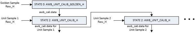
  - Use golden sample and unit sample to capture raw data, and move them to “image” folder in calibration tool path.
  - Open CalibrationInitialParameter.ini file and set parameters of [RAW INFO] section. (Please refer to Section 16.1.2.)
    - Select file path and format of golden sample
    - Set in/out_data_precision to 16
    - Set calibration_select to 2
    - Set load_calibration_data to 0
  - Set parameters of [AWB] section in CalibrationInitialParameter.ini file. (Please refer to Section 16.5.2.)
    - Set CaliState to 0
    - Set CaliNumber to 1
    - Set HighCT to the color temperature of the light source
    - Set OB value. Parameter range: 0 ~ 65535
  - Execute CalibrationRelease.exe to create awb_cali.data containing golden sample calibration result at \data\cfg. Be sure to keep this data until calibration is brought to finish.
  - Open CalibrationInitialParameter.ini file and set parameters of [RAW INFO] section. (Please refer to Section 16.1.2.)
    - Select file path and format of unit sample.
    - Set in/out_data_precision to 16.
    - Set calibration_select to 2.
    - Set load_calibration_data to 1 to keep the data previously calibrated.
  - Set parameters of [AWB] section in CalibrationInitialParameter.ini file. (Please refer to Section 16.5.2.)
    - Set CaliState to 2.
    - Set CaliNumber to 1.
    - Set HighCT to the color temperature value of the light source.
    - Set OB value. Parameter range: 0 ~ 65535.
  - Execute CalibrationRelease.exe to create final awb_cali.data at \data\cfg. If cali_dump_data in [CALI_DB] section is set to 1, a dump_awb_data.txt file will also be created. You can check the calibration result in this txt file.
  - For next unit sample calibration, you can simply load final awb_cali.data from the previous calibration and excute State 2 to replace the unit sample calibration result.
  - Use MI_S32 MI_ISP_API_CmdLoadCaliData API to apply awb_cali.data. (Please refer to SStar_PUDDING_ISP_Software_Development_Guide for details.)
2. The steps for calibration using two light sources are described below:
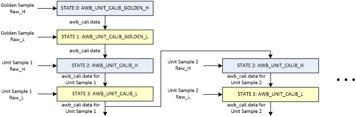
  - Use golden sample and unit sample to capture raw data for two light temperatures, and move them to “image” folder in calibration tool path.
  - Open CalibrationInitialParameter.ini file and set parameters of [RAW INFO] section. (Please refer to Section 16.1.2.)
    - Select file path and format of golden sample high color temperature raw data.
    - Set in/out_data_precision to 16.
    - Set calibration_select to 2.
    - Set load_calibration_data to 0.
  - Set parameters of [AWB] section in CalibrationInitialParameter.ini file. (Please refer to Section 16.5.2.)
    - Set CaliState to 0.
    - Set CaliNumber to 2.
    - Set HighCT to the color temperature of the light source.
    - Set OB value. Parameter range: 0 ~ 65535.
  - Excute CalibrationRelease.exe to create awb_cali.data containing golden sample high color temperature calibration result at \data\cfg. Be sure to keep this data until calibration is brought to finish.
  - Open CalibrationInitialParameter.ini file and set parameters of [RAW INFO] section. (Please refer to Section 16.1.2.)
    - Select file path and format of golden sample low color temperature raw data.
    - Set in/out_data_precision to 16.
    - Set calibration_select to 2.
    - Set load_calibration_data to 1.
  - Set parameters of [AWB] section in CalibrationInitialParameter.ini file. (Please refer to Section 16.5.2.)
    - Set CaliState to 1.
    - Set CaliNumber to 2.
    - Set LowCT to the color temperature of the light source.
    - Set OB value. Parameter range: 0 ~ 65535.
  - Excute CalibrationRelease.exe to create awb_cali.data containing the golden sample color temperature calibration results of the two light sources at \data\cfg. Be sure to keep this data until calibration is brought to finish.
  - Open CalibrationInitialParameter.ini file and set parameters of [RAW INFO] section. (Please refer to Section 16.1.2.)
    - Select file path and format of unit sample high color temperature raw data.
    - Set in/out_data_precision to 16.
    - Set calibration_select to 2.
    - Set load_calibration_data to 1 to keep the data previosly calibrated.
  - Set parameters of [AWB] section in CalibrationInitialParameter.ini file. (Please refer to Section 16.5.2.)
    - Set CaliState to 2.
    - Set CaliNumber to 2.
    - Set HighCT to the color temperature of the light source.
    - Set OB value. Parameter range: 0 ~ 65535.
  - Excute CalibrationRelease.exe to create awb_cali.data containing the golden sample color temperature calibration results of the two light sources and the unit sample high color temperature calibration result at \data\cfg. Be sure to keep this data until calibration is brought to finish.
  - Open CalibrationInitialParameter.ini file and set parameters of [RAW INFO] section. (Please refer to Section 16.1.2.)
    - Select file path and format of unit sample low color temperature raw data.
    - Set in/out_data_precision to 16.
    - Set calibration_select to 2.
    - Set load_calibration_data to 1 to keep the data previously calibrated.
  - Set parameters of [AWB] section in CalibrationInitialParameter.ini file. (Please refer to Section 16.5.2.)
    - Set CaliState to 3.
    - Set CaliNumber to 2.
    - Set LowCT to the color temperature of the light source.
    - Set OB value. Parameter range: 0 ~ 65535.
  - Excute CalibrationRelease.exe to create final awb_cali.data at \data\cfg. If cali_dump_data in [CALI_DB] section is set to 1, a dump_awb_data.txt file will also be created after executing CalibrationRelease.exe. You can check the calibration result in this txt file.
  - For next unit sample calibration, you can simply excute State 2 & 3 to load final awb_cali.data created before and replace the unit sample calibration result.
  - Use MI_ISP_API_CmdLoadCaliData API to apply awb_cali.data. (Please refer to SStar_PUDDING_ISP_Software_Development_Guide for details.)

16.5.4. .data Format and Size¶

Handle size : 20 bytes

Ctrl size : 28 bytes

Data size : 16 bytes

Total size : 20 + 28 + 16 bytes

16.6. SDC Adjustment¶

SDC is used for defective pixel compensation, including black and white point compensation.

16.6.1. Calibration Environment¶

Raw image should be grabbed under a dark environment for white point calibration, just like the required environment for OBC adjustment. For black point calibration, use uniform light source as required by ALSC adjustment.

16.6.2. Parameter Description¶

Item : Selects “0” for grabbing Raw image under darkened environment to calibrate white points; selects “1” for grabbing Raw image with a uniform light source to calibrate black points; selects “2” for grabbing Raw image under the mixed condition.

MixerRatio : The ratio of calibrating white points to black points, only effective when Item = 2.

Ratio value at 100 means taking all the results of Item = 0, while value at 0 means taking all the results of Item = 1.

CaliImgNum : The number of Raw image to be calibrated; this value should be the same with frame_numbers.

InvalidRatio : Sets ratio value for the search range to be filtered out. Parameter range: 1 ~ 100.

CaliFlag : Sets the switch for determining whether cluster of defective pixels in the image should be distinguished. 0 means disable, 1 enable. Parameter range: 0 ~ 1.

ValidValue : Outputs parameter to show the value of defective pixel (in N+1) in the screen after compensation. “N” is the number of compensated defective pixel.

ClusterAmount : Outputs parameter to show the calculated number of cluster when CaliFlag = 1.

TotalAmount : Outputs parameter to show the total number of calibrated pixel point.

16.6.3. Calibration Steps¶

Grabs Raw image to calibrate defective pixels. User can choose from correcting either black points or white points only, while correction of mixed results is also available.
Generates sdc_cali.data. User may also generate dump_sdc_data.txt to view calibration results and then load sdc_cali.data.
Values will not be displayed on IQTool interface.
Please contact SigmaStar if defective pixels fail to be compensated to the extent that white points are still visible under darkened environment or black points still persist with a uniform light source.

16.6.4. .data Format and Size¶

Handle size : 20 bytes

Ctrl size : 44 bytes

Data size : 6144 bytes

Total size : 20 + 44 + 6144 bytes

17. DIFFERENCE WITH MACARON¶

| Module | Function Difference | API Difference (Remove) | API Difference (Add) | |--------------|--------------------------|-----------------------------------| | HDR | Added ghost image compensation function | u16SensorExpRatio
bDynRatioEn
u8CRefSel | u16NoiseLevel[16]
u16MotionTh
u16MotionAdjLut[7] | | HDR Ex | Added ghost image compensation function | | Added associated API | | NR3D | Added a function to reduce dynamic noise stability issue | u16MdThd
u8TfLut[16]
u8YSfStr | u8MdThd
u16TfLut[16]
u8YSfBlendOffset | | NR3D EX | Added noise treatment for purple fringing area Optimized pink ghost image phenomenon at high brightness area | | Added associated API | | Crosstalk | Added a function for adjusting strength by Y | u8StrengthV2
u16ThresholdV2
u16ThresholdOffsetV2 | u8Strength
u8Threshold
u16Offset
u8StrengthByY[15] | | NRDeSpike | Added a function for adjusting DPC strength by diff and Y | u16DiffGainCenterNeighbor
u16DiffThdCornerCross | u8DiffGainCenterNeighbor
u8DiffThdCornerCross
u16BlendLut[5]
u8StrengthByY[15] | | NRLuma | Optimized pre-YNR function | bLumaAdjEn u8LumaX[9]
u16LumaStrByY[10]
u8Wei[20] | u8Strength
u8GMaskSel
u16SpfBlendLut[2] | | NRLuma Adv | Added post-YNR function | | Added associated API | | NRChroma Adv | Added pre-CNR function | | Added associated API | | Sharpness | Optimized high frequency edge sharpness | stEdgeCtrl
stTextureCtrl
u8EdgeKillLUT
bDirEn
u16SharpnessUD
u16SharpnessD | u16EdgeKillLUT
u16SharpnessUD[2]
u16SharpnessD[2]
u8PreCorUD[2]
u8PreCorD[2] u8PreCorMotGain
u8LpfEdgeGainUD
u8LpfEdgeGainD
u8WeakDetailEnhance
u8DetailMotOffset
u8MotGain[16] | | Sharpness Ex | Optimized high frequency edge sharpness | | Added associated API | | PFC | Added defringing function | | Added associated API | | PFC Ex | Added defringing function | | Added associated API |